Another update about using R to analyze the reference desk statistics that we keep at York University Libraries with LibStats (see also Better ways of using R on LibStats (1) and Better ways of using R on LibStats (2): durations, which is about how long we spend helping people at the desk). This is more about time spent, and it rehauls what I wrote up in May 2011 in Ref desk 5: Fifteen minutes for under one per cent. There I said:
Put those two charts together and it shows that during term time we spend on average about fifteen minutes a week giving research help to each of under one per cent of our students.
That’s still true, but now I can calculate it faster and make better charts to show it. And I figure it monthly: weekly showed some nice variations, but monthly is very easy to deal with, and nicely handles the three busy months per term.
As before, I get the data ready.
> library(ggplot2)
> library(dplyr)
> library(lubridate)
> library(scales) # To use better date formatting in axis labels
> l <- read.csv("~/R/yul/libstats/libstats.csv")
> l$day <- as.Date(l$timestamp, format="%m/%d/%Y %r")
> l$month <- floor_date(l$day, "month")
Thanks to a suggestion from Hadley Wickham (whose dplyr and ggplot2 packages I use all the time), I calculate the estimated durations of each encounter by using inner_join from dplyr, which does the same thing as merge but faster and more tidily.
The data frame is too big to look at nicely, so I’ll pick out three columns.
> head(l[c("day", "question.type", "time.spent")])
         day                 question.type    time.spent
1 2011-02-01             4. Strategy-Based  5-10 minutes
2 2011-02-01             4. Strategy-Based 10-20 minutes
3 2011-02-01             4. Strategy-Based  5-10 minutes
4 2011-02-01 3. Skill-Based: Non-Technical  5-10 minutes
5 2011-02-01             4. Strategy-Based  5-10 minutes
6 2011-02-01             4. Strategy-Based  5-10 minutes
I want to add a new column, est.duration, that turns the time.spent column into an estimate of how many minutes each interaction took. 5-10 minutes becomes 8, 10-20 minutes becomes 15, etc. So I make a durations data frame and do an inner_join with l that adds a new column and puts the right value in every row.
> durations <- data.frame(
  time.spent    = c("0-1 minute", "1-5 minutes", "5-10 minutes", "10-20 minutes", "20-30 minutes", "30-60 minutes", "60+ minutes"),
  est.duration  = c( 1, 4, 8, 15, 25, 40, 65)
  )
> durations
     time.spent est.duration
1    0-1 minute            1
2   1-5 minutes            4
3  5-10 minutes            8
4 10-20 minutes           15
5 20-30 minutes           25
6 30-60 minutes           40
7   60+ minutes           65
)
> l <- inner_join(l, durations, by="time.spent")
> head(l[c("day", "question.type", "time.spent", "est.duration")])
         day                 question.type time.spent est.duration
1 2011-02-03               1. Non-Resource 0-1 minute            1
2 2011-02-06 3. Skill-Based: Non-Technical 0-1 minute            1
3 2011-02-11               1. Non-Resource 0-1 minute            1
4 2011-02-16               1. Non-Resource 0-1 minute            1
5 2011-02-17               1. Non-Resource 0-1 minute            1
6 2011-02-17               1. Non-Resource 0-1 minute            1
The rows got reordered, but that doesn’t matter. The est.duration column does actually have the right numbers in it, it’s not just all 1s.
I’ll skip over some of the rest of the preparation, which I explained last time, and get on to figuring out about research questions. First, I use dplyr to make a new data frame that collapses just the research questions into monthly summaries of how many were asked and how long they took.
> research.pm <- l %.% filter(question.type %in% research.questions) %.% group_by(library.name, month) %.% summarise(research.minutes = sum(est.duration, na.rm =TRUE), research.count=n())
> research.pm$year <- format(as.Date(research.pm$month), "%Y")
> research.pm$month.name <- month(research.pm$month, label = TRUE)
> research.pm
Source: local data frame [150 x 6]
Groups: library.name

   library.name      month research.minutes research.count year month.name
1      Bronfman 2011-02-01             3670            240 2011        Feb
2      Bronfman 2011-03-01             4035            294 2011        Mar
3      Bronfman 2011-04-01             1292             92 2011        Apr
4      Bronfman 2011-05-01              725             59 2011        May
5      Bronfman 2011-06-01              903             77 2011        Jun
6      Bronfman 2011-07-01              554             46 2011        Jul
7      Bronfman 2011-08-01              296             27 2011        Aug
8      Bronfman 2011-09-01             1057             87 2011        Sep
9      Bronfman 2011-10-01             2163            182 2011        Oct
10     Bronfman 2011-11-01             4037            281 2011        Nov
..          ...        ...              ...            ...  ...        ...
> ggplot(research.pm, aes(x=year, y=research.count)) + geom_bar(stat="identity") + facet_grid(library.name ~ month.name) + labs(x="", y="", title="Research questions per month (year to year)") + theme(axis.text.x = element_text(angle = 90))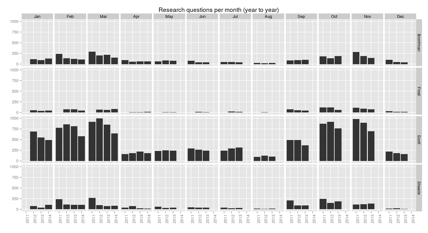
Slight decline in the numbers of research questions asked each month, year to year. Why? I don’t know. We need to investigate.
(The images look a bit grotty because I shrank them down, but each is a link to a full-size version.)
> ggplot(research.pm, aes(x=year, y=research.minutes/60)) + geom_bar(stat="identity") + facet_grid(library.name ~ month.name) + labs(x="", y="Hours", title="Hours of research support (year to year)") + theme(axis.text.x = element_text(angle = 90))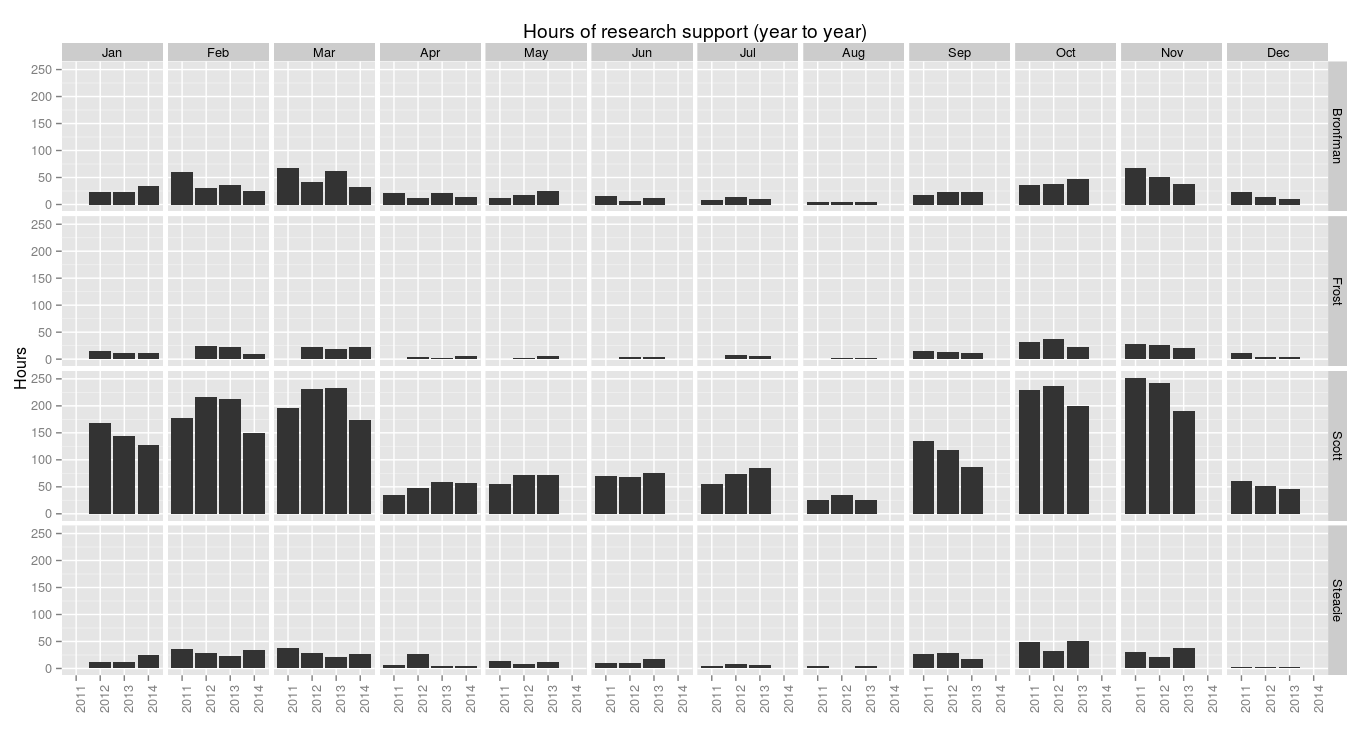
This shows that sometimes fewer quesions doesn’t mean less time spent helping people with research. But knowing how many questions were asked and how long they all took, it’s trivial to divide to find the average.
> ggplot(research.pm, aes(x=year, y=research.minutes/research.count)) + geom_bar(stat="identity") + facet_grid(library.name ~ month.name) + labs(x="", y="Minutes", title="Average length of research help sessions (year to year)") + theme(axis.text.x = element_text(angle = 90))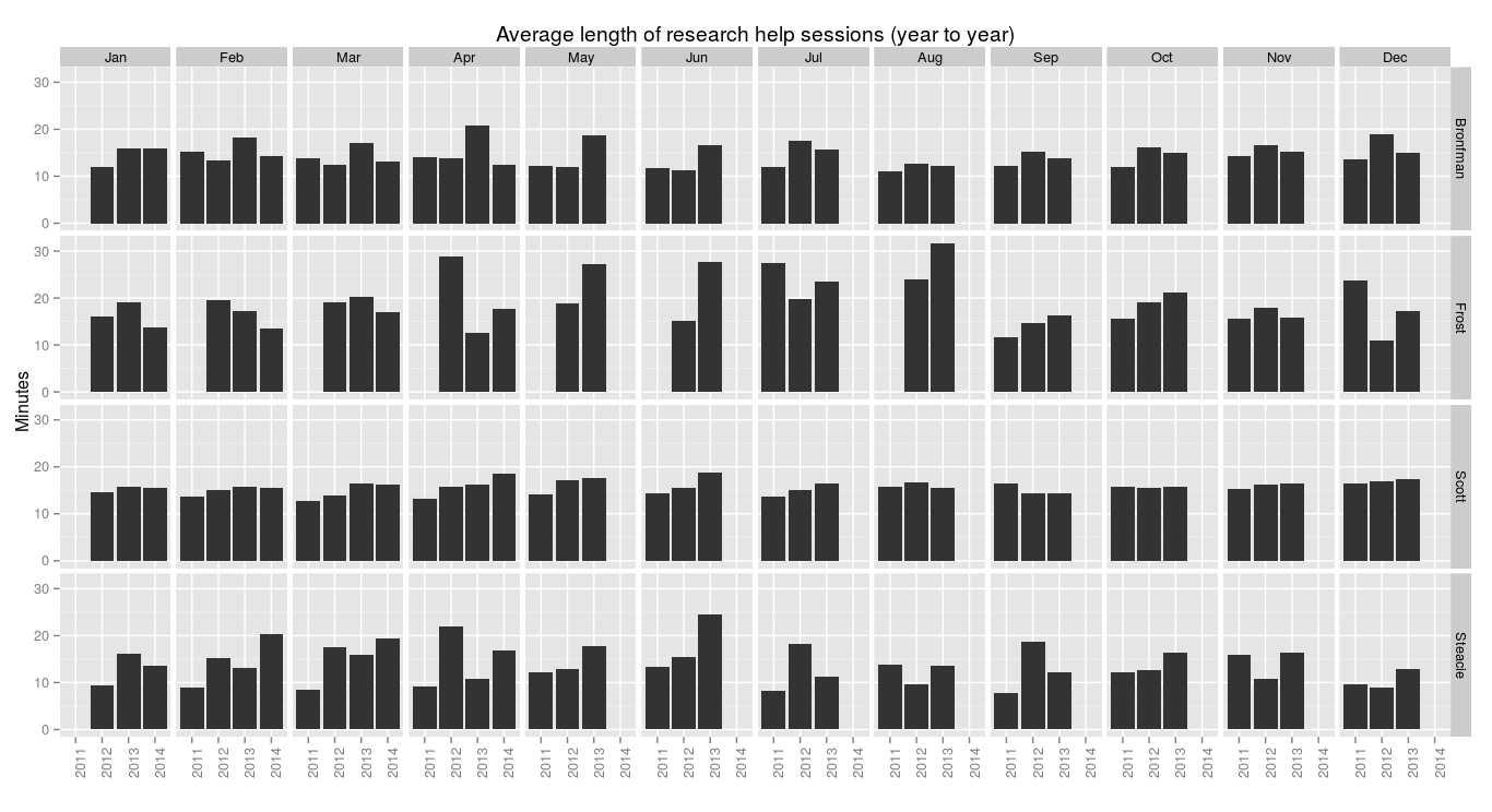
Some variation there among the smaller branches, but Scott, which has the most students and is by far the busiest, stays very consistent at 15–20 minutes per research help session.
I explained in another post about “home users,” the number of students that (in theory) use a given library—this should be especially true for research questions—and here I set up a data frame with the branch names and numbers for each year.
> years=c(2011:2014)
> home.users <- rbind(
   data.frame(library.name="Bronfman", academic.year=years, users=c( 6007,  5991,  6050,  6295)),
   data.frame(library.name="Frost",    academic.year=years, users=c( 2655,  2672,  2677,  2671)),
   data.frame(library.name="Scott",    academic.year=years, users=c(33577, 34321, 34388, 33852)),
   data.frame(library.name="Steacie",  academic.year=years, users=c( 9576,  9858, 10018, 10394))
   )
> home.users
   library.name academic.year users
1      Bronfman          2011  6007
2      Bronfman          2012  5991
3      Bronfman          2013  6050
4      Bronfman          2014  6295
5         Frost          2011  2655
6         Frost          2012  2672
7         Frost          2013  2677
8         Frost          2014  2671
9         Scott          2011 33577
10        Scott          2012 34321
11        Scott          2013 34388
12        Scott          2014 33852
13      Steacie          2011  9576
14      Steacie          2012  9858
15      Steacie          2013 10018
16      Steacie          2014 10394
Before we match things up we need to align things by academic year. Academic 2013–2014, which I’d label 2014, started last May (2013-05-01) and ends today (2014-04-30). An easy way to calculate the academic year of a given date is to push it ahead by as many days separate 1 May from 1 January and then use the year of the resulting date. Anything from January to April stays in the same year, but everything later gets knocked ahead a year.
> as.Date("2014-01-01") - as.Date("2013-05-01")
Time difference of 245 days
> as.Date("2014-04-30") + 245
[1] "2014-12-31"
> as.Date("2014-05-01") + 245
[1] "2015-01-01"
> research.pm$academic.year <- as.integer(format(research.pm$month+245, "%Y"))
> Source: local data frame [150 x 7]
Groups: library.name

   library.name      month research.minutes research.count year month.name academic.year
1      Bronfman 2011-02-01             3670            240 2011        Feb          2011
2      Bronfman 2011-03-01             4035            294 2011        Mar          2011
3      Bronfman 2011-04-01             1292             92 2011        Apr          2011
4      Bronfman 2011-05-01              725             59 2011        May          2012
5      Bronfman 2011-06-01              903             77 2011        Jun          2012
6      Bronfman 2011-07-01              554             46 2011        Jul          2012
7      Bronfman 2011-08-01              296             27 2011        Aug          2012
8      Bronfman 2011-09-01             1057             87 2011        Sep          2012
9      Bronfman 2011-10-01             2163            182 2011        Oct          2012
10     Bronfman 2011-11-01             4037            281 2011        Nov          2012
..          ...        ...              ...            ...  ...        ...           ...
> research.pm <- inner_join(research.pm, home.users, by=c("library.name", "academic.year"))
> research.pm
Source: local data frame [150 x 8]
Groups: library.name

   library.name      month research.minutes research.count year month.name academic.year users
1      Bronfman 2011-02-01             3670            240 2011        Feb          2011  6007
2      Bronfman 2011-03-01             4035            294 2011        Mar          2011  6007
3      Bronfman 2011-04-01             1292             92 2011        Apr          2011  6007
4      Bronfman 2011-05-01              725             59 2011        May          2012  5991
5      Bronfman 2011-06-01              903             77 2011        Jun          2012  5991
6      Bronfman 2011-07-01              554             46 2011        Jul          2012  5991
7      Bronfman 2011-08-01              296             27 2011        Aug          2012  5991
8      Bronfman 2011-09-01             1057             87 2011        Sep          2012  5991
9      Bronfman 2011-10-01             2163            182 2011        Oct          2012  5991
10     Bronfman 2011-11-01             4037            281 2011        Nov          2012  5991
..          ...        ...              ...            ...  ...        ...           ...   ...
> ggplot(research.pm, aes(x=year, y=100*research.count/users)) + geom_bar(stat="identity") + facet_grid(library.name ~ month.name) + labs(x="", y="%", title="Home users seen about research") + theme(axis.text.x = element_text(angle = 90))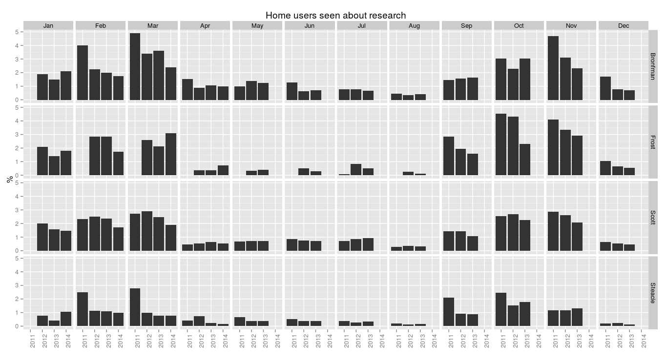
Assuming each research question is asked by a different person, this shows that each month we see 2-3% of home users about research. Of course, if some people ask more than one question, that ratio is lower. (There is research underway to find out who these users are—the hypothesis is that it isn’t 3% of all students that get research help, but a much higher proportion of a much smaller set of students: who are they, what kind of help do they need, and how can we change what we offer to be of more use?) I’m curious about the situation at other libraries and what their numbers show.
Two years ago I said:
Put those two charts together and it shows that during term time we spend on average about fifteen minutes a week giving research help to each of under one per cent of our students.
Now I say: “During term time each month we give about fifteen minutes of research support to two or three per cent of our students.”
> ggplot(research.pm, aes(x=year, y=100*research.count/users)) + geom_bar(stat="identity") + facet_grid(library.name ~ month.name) + labs(x="", y="%", title="Home users seen about research") + theme(axis.text.x = element_text(angle = 90))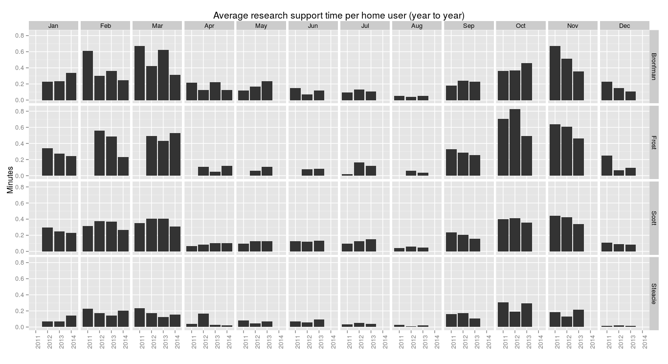
On average, each home user gets under one minute of research support each month. Again, this isn’t how it actually works—a smaller percentage of users get more help, though we don’t know the details yet—but again I’m curious to know how this compares to other libraries.
That’s it for the R and library stats posts for now, I think. Try dplyr, it’s great.