A couple of years ago I wrote some R scripts to analyze the reference desk statistics that we keep at York University Libraries with LibStats. I wrote five posts here about what I found; the last one, Ref desk 5: Fifteen minutes for under one per cent, links to the other four.
Those scripts did their job, but they were ugly, and there were some more things I wanted to do. Because of my recent Ubuntu upgrade, I’m running R version 3.0.2 now, which means I can use the new dplyr package by R wizard Hadley Wickham and others. (It doesn’t work on 3.0.1.) The vignette for dplyr has lots of examples, and I’ve been seeing great posts about it, and I was eager to try it. So I’m going back to the old work and refreshing it and figuring out how to do what I wanted to do in 2012—or couldn’t because we only had one year of data; now that we have four, year-to-year comparisons are interesting.
This first post is about how I used to do things in an ugly and slow way, and how to do them faster and better.
I begin with a CSV file containing a slightly munged and cleaned dump of all the information from LibStats.
$ head libstats.csv
timestamp,question.type,question.format,time.spent,library.name,location.name,initials
02/01/2011 09:20:11 AM,4. Strategy-Based,In-person,5-10 minutes,Scott,Drop-in Desk,AA
02/01/2011 09:43:09 AM,4. Strategy-Based,In-person,10-20 minutes,Scott,Drop-in Desk,AA
02/01/2011 10:00:56 AM,4. Strategy-Based,In-person,5-10 minutes,Scott,Drop-in Desk,AA
02/01/2011 10:05:05 AM,3. Skill-Based: Non-Technical,Phone,5-10 minutes,Scott,Drop-in Desk,AA
02/01/2011 10:17:20 AM,4. Strategy-Based,In-person,5-10 minutes,Scott,Drop-in Desk,AA
02/01/2011 10:30:07 AM,4. Strategy-Based,In-person,5-10 minutes,Scott,Drop-in Desk,AA
02/01/2011 10:54:41 AM,4. Strategy-Based,In-person,5-10 minutes,Scott,Drop-in Desk,AA
02/01/2011 11:08:00 AM,4. Strategy-Based,In-person,10-20 minutes,Scott,Drop-in Desk,AA
02/01/2011 11:32:00 AM,3. Skill-Based: Non-Technical,In-person,10-20 minutes,Scott,Drop-in Desk,AA
I read the CSV file into a data frame, then fix a couple of things. The date is a string and needs to be turned into a Date, and I use a nice function from lubridate to find the floor of the date, which aggregates everything to the month it’s in.
> l <- read.csv("libstats.csv")
> library(lubridate)
> l$day <- as.Date(l$timestamp, format="%m/%d/%Y %r")
> l$month <- floor_date(l$day, "month")
> str(l)
'data.frame':	187944 obs. of  9 variables:
 $ timestamp      : chr  "02/01/2011 09:20:11 AM" "02/01/2011 09:43:09 AM" "02/01/2011 10:00:56 AM" "02/01/2011 10:05:05 AM" ...
 $ question.type  : chr  "4. Strategy-Based" "4. Strategy-Based" "4. Strategy-Based" "3. Skill-Based: Non-Technical" ...
 $ question.format: chr  "In-person" "In-person" "In-person" "Phone" ...
 $ time.spent     : chr  "5-10 minutes" "10-20 minutes" "5-10 minutes" "5-10 minutes" ...
 $ library.name   : chr  "Scott" "Scott" "Scott" "Scott" ...
 $ location.name  : chr  "Drop-in Desk" "Drop-in Desk" "Drop-in Desk" "Drop-in Desk" ...
 $ initials       : chr  "AA" "AA" "AA" "AA" ...
 $ day            : Date, format: "2011-02-01" "2011-02-01" "2011-02-01" "2011-02-01" ...
 $ month          : Date, format: "2011-02-01" "2011-02-01" "2011-02-01" "2011-02-01" ...
> head(l)
               timestamp                 question.type question.format    time.spent library.name location.name initials
1 02/01/2011 09:20:11 AM             4. Strategy-Based       In-person  5-10 minutes        Scott  Drop-in Desk       AA
2 02/01/2011 09:43:09 AM             4. Strategy-Based       In-person 10-20 minutes        Scott  Drop-in Desk       AA
3 02/01/2011 10:00:56 AM             4. Strategy-Based       In-person  5-10 minutes        Scott  Drop-in Desk       AA
4 02/01/2011 10:05:05 AM 3. Skill-Based: Non-Technical           Phone  5-10 minutes        Scott  Drop-in Desk       AA
5 02/01/2011 10:17:20 AM             4. Strategy-Based       In-person  5-10 minutes        Scott  Drop-in Desk       AA
6 02/01/2011 10:30:07 AM             4. Strategy-Based       In-person  5-10 minutes        Scott  Drop-in Desk       AA
The columns are:
- timestamp: timestamp (not in a standard format)
- question.type: one of five categories of question (1 = directional, 5 = specialized)
- question.format: how or where the question was asked (in person, phone, chat)
- time.spent: time spent giving help
- library.name: the library name
- location.name: where in the library (ref desk, office, info desk)
- initials: initials of the person (or people) who helped
Now I have these fields in the data frame that I will use:
> head(subset(l, select=c("day", "month", "question.type", "time.spent", "library.name")))
         day      month                 question.type    time.spent library.name
1 2011-02-01 2011-02-01             4. Strategy-Based  5-10 minutes        Scott
2 2011-02-01 2011-02-01             4. Strategy-Based 10-20 minutes        Scott
3 2011-02-01 2011-02-01             4. Strategy-Based  5-10 minutes        Scott
4 2011-02-01 2011-02-01 3. Skill-Based: Non-Technical  5-10 minutes        Scott
5 2011-02-01 2011-02-01             4. Strategy-Based  5-10 minutes        Scott
6 2011-02-01 2011-02-01             4. Strategy-Based  5-10 minutes        Scott
But I’m going to just take a sample of all of this data, because this is just for illustrative purposes, not real analysis. Let’s grab 10,000 random entries from this data frame and put that into l.sample.
> l.sample <- l[sample(nrow(l), 10000),]An easy thing to ask first is: How many questions are asked each month in each library?
Here’s how I did it before. I’ll run the command and show the resulting data frame. I used the plyr package, which is (was) great, and its ddply function, which applies a function to a data frame and gives a data frame back. Here I have it collapse the data frame l along the two columns specified (month and library.name) and use nrow to count how many rows result. Then I check how long it would take to perform that operation on the entire data set.
> library(plyr)
> sample.allquestions.pm <- ddply(l.sample, .(month, library.name), nrow)
> head(sample.allquestions.pm)
       month      library.name  V1
1 2011-02-01          Bronfman  63
2 2011-02-01             Scott  60
3 2011-02-01 Scott Information 183
4 2011-02-01              SMIL  57
5 2011-02-01           Steacie  57
6 2011-03-01          Bronfman  46
> system.time(allquestions.pm <- ddply(l, .(month, library.name), nrow))
   user  system elapsed
  2.812   0.518   3.359
The system.time line there show how long the previous command takes to run on the entire data frame: almost 3.5 seconds! That is slow. Do a few of those, chopping and slicing the data in various ways, and it will really add up.
This is a bad way of doing it. It works! But it’s slow and I wasn’t thinking about the problem the right way. Using ddply and nrow was wrong: I should have been using count (also from plyr), which I wrote up a while back, with some examples. That’s a much faster and more sensible way of counting up the number of rows in a data set.
But now that I can use dplyr, I can approach the problem in a whole new way.
First, I’ll clear plyr out of the way, then load dplyr. Doing it this way means no function names collide.
> search()
 [1] ".GlobalEnv"        "package:plyr"      "package:lubridate" "package:ggplot2"   "ESSR"              "package:stats"     "package:graphics"  "package:grDevices"
 [9] "package:utils"     "package:datasets"  "package:methods"   "Autoloads"         "package:base"
> detach("package:plyr")
> library(dplyr)
See how nicely you can construct and chain operations with dplyr:
> l.sample %.% group_by(month, library.name) %.% summarise(count=n())
Source: local data frame [277 x 3]
Groups: month

        month      library.name count
1  2011-02-01          Bronfman    63
2  2011-02-01              SMIL    57
3  2011-02-01             Scott    60
4  2011-02-01 Scott Information   183
5  2011-02-01           Steacie    57
6  2011-03-01          Bronfman    46
7  2011-03-01              SMIL    59
8  2011-03-01             Scott    71
9  2011-03-01 Scott Information   220
10 2011-03-01           Steacie    61
..        ...               ...   ...
The %.% operator lets you chain together different operations, and just for the sake of clarity of reading, I like to arrange things so first I specify the data frame on its own and then walk through the things I do to it. First, group_by breaks down the data frame by columns and does some magic. Then summarise collapses the different chunks of resulting data into one line each, and I use count=n() to make a new column, count, which contains the count of how many rows there were in each chunk, calculated with the n() function. In English I’m saying, “take the l data frame, group it by month and library.name, and count how many rows are in each grouping.” (Also, notice I didn’t need to use the head command to stop it running off the screen, it made it nicely readable on its own.)
It’s easier to think about, it’s easier to read, it’s easier to play with … and it’s much faster. How long would this take to run on the entire data set?
> system.time(l %.% group_by(month, library.name) %.% summarise(count=n()))
   user  system elapsed
  0.032   0.000   0.033
0.03 seconds elapsed time! That is 0.9% of the 3.35 seconds the old way.
Graphing it is easy, using Hadley Wickham’s marvellous ggplot2 package.
> library(ggplot2)
> sample.allquestions.pm <- l.sample %.% group_by(month, library.name) %.% summarise(count=n())
> ggplot(sample.allquestions.pm, aes(x=month, y=count)) + geom_bar(stat="identity") + facet_grid(library.name ~ .) + labs(x="", y="", title="All questions")
> ggsave(filename="20140422-all-questions-1.png", width=8.33, dpi=72, units="in")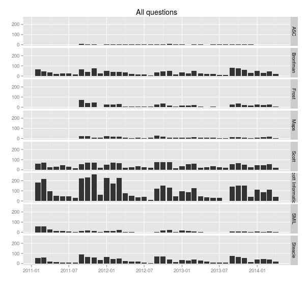
You can see the ebb and flow of the academic year: September, October and November are very busy, then things quiet down in December, then January, February and March busy, then it cools off in April and through the summer. (Students don’t ask a lot of questions close to and during exam time—they’re studying, and their assignments are finished.)
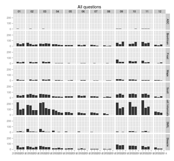
What about comparing year to year? Here’s a nice way of doing that.
First, pick out the numbers of the months and years. The format command knows all about how to handle dates and times. See the man page for strptime or your favourite language’s date manipulation commands for all the options possible. Here I use %m to find the month number and %Y to find the four-digit year. Two examples, then the commands:
> format(as.Date("2014-04-22"), "%m")
[1] "04"
> format(as.Date("2014-04-22"), "%Y")
[1] "2014"
> sample.allquestions.pm$mon  <- format(as.Date(sample.allquestions.pm$month), "%m")
> sample.allquestions.pm$year <- format(as.Date(sample.allquestions.pm$month), "%Y")
> head(sample.allquestions.pm)
Source: local data frame [6 x 5]
Groups: month

       month      library.name count mon year
1 2011-02-01          Bronfman    63  02 2011
2 2011-02-01              SMIL    57  02 2011
3 2011-02-01             Scott    60  02 2011
4 2011-02-01 Scott Information   183  02 2011
5 2011-02-01           Steacie    57  02 2011
6 2011-03-01          Bronfman    46  03 2011
> ggplot(sample.allquestions.pm, aes(x=year, y=count)) + geom_bar(stat="identity") + facet_grid(library.name ~ mon) + labs(x="", y="", title="All questions")
> ggsave(filename="20140422-all-questions-2.png", width=8.33, dpi=72, units="in")
This plot changes the x-axis to the year, and facets along two variables, breaking the the chart up vertically by library and horizontally by month. It’s easy now to see how months compare to each other across years.
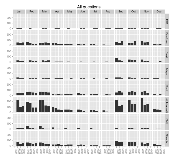
With a little more work we can rotate the x-axis labels so they’re readable, and put month names along the top. The month function from lubridate makes this easy.
> sample.allquestions.pm$month.name <- month(sample.allquestions.pm$month, label = TRUE)
> head(sample.allquestions.pm)
Source: local data frame [6 x 6]
Groups: month

       month      library.name count mon year month.name
1 2011-02-01          Bronfman    63  02 2011        Feb
2 2011-02-01              SMIL    57  02 2011        Feb
3 2011-02-01             Scott    60  02 2011        Feb
4 2011-02-01 Scott Information   183  02 2011        Feb
5 2011-02-01           Steacie    57  02 2011        Feb
6 2011-03-01          Bronfman    46  03 2011        Mar
> ggplot(sample.allquestions.pm, aes(x=year, y=count)) + geom_bar(stat="identity") + facet_grid(library.name ~ month.name) + labs(x="", y="", title="All questions") + theme(axis.text.x = element_text(angle = 90))
> ggsave(filename="20140422-all-questions-3.png", width=8.33, dpi=72, units="in")