3d printing a Sierpinski tetrix
Late last year I got a MakerBot Replicator Mini at work for some research I’m doing. I’ve been printing off some science and math things from Thingiverse, most recently four iterations built from this customizable Sierpinski tetrix.
A Sierpinski tetrix is the three-dimensional analogue of Sierpinski triangle, which is a fractal shape generated by taking a triangle, dividing it into four equal smaller triangles, removing the the middle one, then repeating the operation on each of the three remaining triangles, and so on, forever. You end up with a shape that has a finite (and always constant) perimeter, zero area (!), and a dimension of 1.585 (less than the two-dimensional figure it seems to be). That’s pretty wild.
The Wikipedia and Wolfram MathWorld articles explain more and have diagrams and math. Here are some pictures of what I printed.
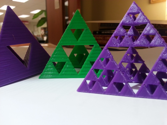
With the tetrix, you start with a tetrahedron, divide it up and remove the middle bit so you have four equal smaller tetrahedra, as shown on the left. Repeat the process with each of the four tetrahedra and you get 16 (4^2) smaller tetrahedra, as shown in the middle. Repeat again to the third iteration and you have 64 (4^3) smaller tetrahedra, as shown on the right.
At the limit you end up with a shape with a constant surface area (unchanged through each iteration), zero volume (!), and 2 dimensions (!!). You can’t print to an infinite level of detail on this printer, which is understandable, but it turns out you can’t reliably print to the fourth iteration, either.
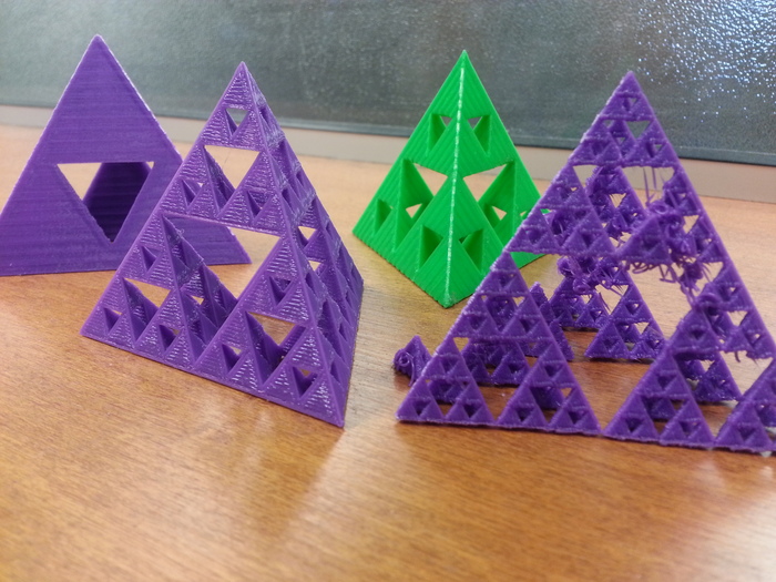
There are supposed to be 256 (4^4) little tetrahedra in that one on the right, but it glitched up while printing and went wonky, and then it broke apart when I removed the supporting material from the sides. It took over five hours to print.
I’ll try again (and I’d like to try it on a better printer) but if that doesn’t work I can print three more level-3 iterations and put them together, because you don’t have to make a big thing smaller, you can also make small things bigger.
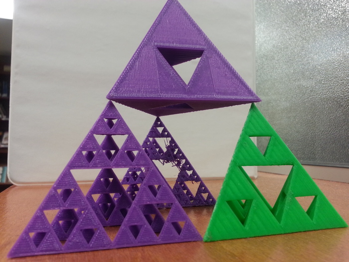
I like the malformed fourth iteration … it looks like the ruin of a futuristic building, decayed after the nanobots that maintained it lost their energy and weird climate change-adapted vines started to grow.
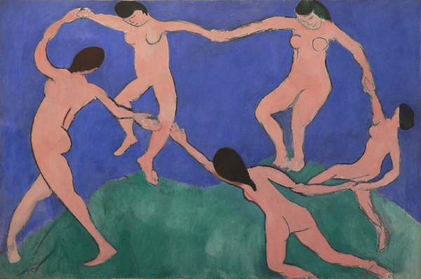
The best paper I read this year: Polster, Reconfiguring the Academic Dance
The best paper I read this year is Reconfiguring the Academic Dance: A Critique of Faculty’s Responses to Administrative Practices in Canadian Universities by Claire Polster, a sociologist at the University of Regina, in Topia 28 (Fall 2012). It’s aimed at professors but public and academic librarians should read it.
Unfortunately, it’s not gold open access. There’s a two year rolling wall and it’s not out of it yet (but I will ask—it should have expired by now). If you don’t have access to it, try asking a friend or following the usual channels. Or wait. Or pay six bucks. (Six bucks? What good does that do, I wonder.)
Update on 04 January 2015: Good news! The paper is now out from the paywall, so it’s freely available to everyone.
Here’s the abstract:
This article explores and critiques Canadian academics’ responses to new administrative practices in a variety of areas, including resource allocation, performance assessment and the regulation of academic work. The main argument is that, for the most part, faculty are responding to what administrative practices appear to be, rather than to what they do or accomplish institutionally. That is, academics are seeing and responding to these practices as isolated developments that interfere with or add to their work, rather than as reorganizers of social relations that fundamentally transform what academics do and are. As a result, their responses often serve to entrench and advance these practices’ harmful effects. This problem can be remedied by attending to how new administrative practices reconfigure institutional relations in ways that erode the academic mission, and by establishing new relations that better serve academics’—and the public’s—interests and needs. Drawing on the work of various academic and other activists, this article offers a broad range of possible strategies to achieve the latter goal. These include creating faculty-run “banks” to transform the allocation of institutional resources, producing new means and processes to assess—and support—academic performance, and establishing alternative policy-making bodies that operate outside of, and variously interrupt, traditional policy-making channels.
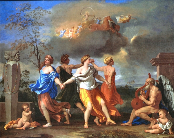
This is the dance metaphor:
To offer a simplified analogy, if we imagine the university as a dance floor, academics tend to view new administrative practices as burdensome weights or shackles that are placed upon them, impeding their ability to perform. In contrast, I propose we see these practices as obstacles that are placed on the dance floor and reconfigure the dance itself by reorganizing the patterns of activity in and through which it is constituted. I further argue that because most academics do not see how administrative practices reorganize the social relations within which they themselves are implicated, their reactions to these practices help to perpetuate and intensify these transformations and the difficulties they produce. Put differently, most faculty do not realize that they can and should resist how the academic dance is changing, but instead concentrate on ways and means to keep on dancing as best they can.
About the constant struggle for resources:
Instead of asking administrators for the resources they need and explaining why they need them, faculty are acting more as entrepreneurs, trying to convince administrators to invest resources in them and not others. One means to this end is by publicizing and promoting ways they comply with administrators’ desires in an ever growing number of newsletters, blogs, magazines and the like. Academics are also developing and trying to “sell” to administrators new ideas that meet their needs (or make them aware of needs they didn’t realize they had), often with the assistance of expensive external consultants. Ironically, these efforts to protect or acquire resources often consume substantial resources, intensifying the very shortages they are designed to alleviate. More importantly, these responses further transform institutional relations, fundamentally altering, not merely adding to, what academics do and what they are.
About performance assessment:
Another academic strategy is to respect one’s public-serving priorities but to translate accomplishments into terms that satisfy administrators. Accordingly, one might reframe work for a local organization as “research” rather than community service, or submit a private note of appreciation from a student as evidence of high-quality teaching. This approach extends and normalizes the adoption of a performative calculus. It also feeds the compulsion to prove one’s value to superiors, rather than to engage freely in activities one values.
Later, when she covers the many ways people try to deal with or work around the problems on their own:
There are few institutional inducements for faculty to think and act as compliant workers rather than autonomous professionals. However, the greater ease that comes from not struggling against a growing number of rules, and perhaps the additional time and resources that are freed up, may indirectly encourage compliance.
Back to the dance metaphor:
If we return to the analogy provided earlier, we may envision academics as dancers who are continually confronted with new obstacles on the floor where they move. As they come up to each obstacle, they react—dodging around it, leaping over it, moving under it—all the while trying to keep pace, appear graceful and avoid bumping into others doing the same. It would be more effective for them to collectively pause, step off the floor, observe the new terrain and decide how to resist changes in the dance, but their furtive engagement with each obstacle keeps them too distracted to contemplate this option. And so they keep on moving, employing their energies and creativity in ways that further entangle them in an increasingly difficult and frustrating dance, rather than trying to move in ways that better serve their own—and others’ —needs.
She with a number of useful suggestions about how to change things, and introduces this by saying:
Because so many academic articles are long on critique but short on solutions, I present a wide range of options, based on the reflections and actions of many academic activists both in the past and in the present, which can challenge and transform university relations in positive ways.
Every paragraph hit home. At York University, where I work, we’re going through a prioritization process using the method set out by Robert Dickeson. It’s being used at many universities, and everything about it is covered by Polster’s article. Every reaction she lists, we’ve had. Also, the university is moving to activity-based costing, a sort of internal market system, where some units (faculties) bring in money (from tuition) and all the other units (including the libraries) don’t, and so are cost centres. Cost centres! This has got people in the libraries thinking about how we can generate revenue. Becoming a profit centre! A university library! If thinking like that gets set in us deep the effects will be very damaging.
Animated intersecting circles
I was looking again at some of the intersecting circles I wrote about last month, looking at 2, 3, 4, 5, 6 intersecting circles one after the other, and it looked pretty smart, so I tried making an animated GIF out of it. The R package animation makes it pretty easy.
Here’s the setup, which gives the drawcircles function.
circle <- function(x, y, rad = 1.1, vertices = 500, ...) {
  rads <- seq(0, 2*pi, length.out = vertices)
  xcoords <- cos(rads) * rad + x
  ycoords <- sin(rads) * rad + y
  polygon(xcoords, ycoords, ...)
}

roots <- function(n) {
  lapply(
    seq(0, n - 1, 1),
    function(x)
      c(round(cos(2*x*pi/n), 4), round(sin(2*x*pi/n), 4))
  )
}

drawcircles <- function(n) {
  centres <- roots(n)
  plot(-2:2, type="n", xlim = c(-2,2), ylim = c(-2,2), asp = 1, xlab = "", ylab = "", axes = FALSE)
  lapply(centres, function (c) circle(c[[1]], c[[2]]))
}> 1:10
[1] 1 2 3 4 5 6 7 8 9 10
> 9:2
[1] 9 8 7 6 5 4 3 2
> c(1:10, 9:2)
[1] 1 2 3 4 5 6 7 8 9 10 9 8 7 6 5 4 3 2> library(animation)
> saveGIF({for (i in c(1:60, 59:2)) drawcircles(i)}, interval = 0.2, movie.name = "intersecting-circles.gif")
The GIF is 2.1 MB, which is pretty large. Perhaps there’s some way to make a smaller file. In any case, it’d be nice to see that projected on a huge wall. Nice vids.
Reading diary in Org
Last year I started using Org to keep track of my reading, instead of on paper, and it worked very well. I was able to see how much I was reading all through the year, which helped me read more.
I have two tables. The first is where I enter what I read. For each book I track the start date, title, author, number of pages, and type (F for fiction, N for nonfiction, A for article). If I don’t finish a book or just skim it I leave the pages field blank and put a - in T. Today I started a new book so there’s just one title, but to add a new one I would go to the dashed line at the bottom and hit S-M-<down> (that’s Alt-Shift-<down> in Emacs-talk) and it creates a new formatted line. I’m down at the bottom of the table so I tab through a few times to get to the # line, which forces a recalculation of the totals.
#+CAPTION: 2015 reading diary
#+ATTR_LATEX: :environment longtable :align l|p{8cm}|p{ccm}|l|l
#+NAME: reading_2015
|   | Date        | Title                              | Author            | Pages | T |
|   |             | <65>                               | <40>              |       |   |
|---+-------------+------------------------------------+-------------------+-------+---|
|   | 01 Jan 2015 | Stoicism and the Art of Happiness  | Donald Robertson  |   232 | N |
|---+-------------+------------------------------------+-------------------+-------+---|
| # |             | 1                                  |                   |   232 |   |
#+TBLFM: $3=@#-3::$5=vsum(@3..@-1)
(The #+CAPTION and #+ATTR_LATEX lines are for the LaTeX export I use if I want to print it.)
The second table is all generated from the first one. I tab through it to refresh all the fields. All of the formulas in the #+TBLFM field should be on one line, but I broke it out here to make it easier to read.
Books per week and predicted books per year are especially helpful in keeping me on track.
#+NAME: reading-analysis-2015
#+CAPTION: 2015 reading statistics
|---+----------------------+---------------|
|   | Statistic            |               |
|---+----------------------+---------------|
| # | Fiction books        |             0 |
| # | Nonfiction books     |             1 |
| # | Articles             |             0 |
| # | DNF or skimmed       |             0 |
| # | Total books read     |             1 |
| # | Total pages read     |           232 |
| # | Days in              |           001 |
| # | Weeks in             |            00 |
| # | Books per week       |             1 |
| # | Pages per day        |           232 |
| # | Predicted books/year |           365 |
|---+----------------------+---------------|
#+TBLFM: @2$3='(length(org-lookup-all "F" '(remote(reading_2015,@2$6..@>$6)) nil))::
@3$3='(length(org-lookup-all "N" '(remote(reading_2015,@2$6..@>$6)) nil))::
@4$3='(length(org-lookup-all "A" '(remote(reading_2015,@2$6..@>$6)) nil))::
@5$3='(length(org-lookup-all "-"  '(remote(reading_2015,@2$6..@>>$6)) nil));E::
@6$3=@2$3+@3$3::@7$3=remote(reading_2015, @>$5)::
@8$3='(format-time-string "%j")::
@9$3='(format-time-string "%U")::
@10$3=round(@6$3/@9$3, 1)::
@11$3=round(@7$3/@8$3, 0)::
@12$3=round(@6$3*365/@8$3, 0)
(Tables and the spreadsheet in Org are very, very useful. I use them every day for a variety of things.)
With all that information in tables it’s easy to embed code to pull out other statistics and make charts. I’ll cover that when I tweak something to handle co-written books, but today, after getting some of that working for the first time, I was able to see my most read authors over the last four years are Anthony Trollope, Terry Pratchett and Anthony Powell. There are 39 authors who I’ve read at least twice. Some of them I’ll never read again, some I’ll read everything new they come out with (like Sarah Waters, who I only started reading this year) and some are overdue for rereading (like Georgette Heyer).
CBC appearances (updated)
Sean Craig’s Amanda Lang took money from Manulife & Sun Life, gave them favourable CBC coverage piece on Canadaland got me looking at the cbcappearances script I wrote earlier this year.
It wasn’t getting any of the recent appearances—looks like the CBC changed how they are storing the data that is presented: instead of pulling it in on the fly from Google spreadsheets, it’s all the page in a hidden table (generated by their content management system, I guess) and shown as needed.
They should be making the data available in a reusable format, but they still aren’t. So we need to scrape it, but that’s easy, so I updated the script and regenerated appearances.csv, a nice reusable CSV file suitable for importing into your favourite data analysis tool. The last appearance listed was on 29 November 2014; I assume the December ones will show up soon in January.
The data shows 218 people have made 716 appearances since 24 April 2014. A quick histogram of appearances per person shows that most made only 1 or 2 appearances, and then it quickly tails off. Here how I did things in R:
> library(dplyr)
> library(ggplot2)
> cbc <- read.csv("appearances.csv", header = TRUE, stringsAsFactors = TRUE)
> cbc$date <- as.Date(cbc$date)
> totals <- cbc %>% group_by(name) %>% summarise(count = n()) %>% select(count)
> qplot(totals$count, binwidth = 1)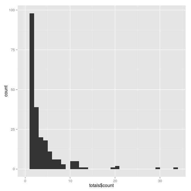
The median number of appearances is 2, the mean is about 3.3, and third quartile is 4 and above. Let’s label anyone in the third quartile as “busy,” and pick out everyone who is busy, then make a data frame of just the appearance information about busy people.
> summary(totals$count)
   Min. 1st Qu.  Median    Mean 3rd Qu.    Max.
  1.000   1.000   2.000   3.284   4.000  33.000
> quantile(totals$count)
  0%  25%  50%  75% 100%
  1    1    2    4   33
> busy.number <- quantile(totals$count)[[4]]
> busy.number
[1] 4
> busy_people <- cbc %>% group_by(name) %>% summarise(count = n()) %>% filter(count >= busy.number) %>% select(name)
> head(busy_people)
Source: local data frame [6 x 1]

                 name
1     Adrian Harewood
2           Alan Neal
3         Amanda Lang
4        Andrew Chang
5 Anne-Marie Mediwake
6       Brian Goldman
> busy <- a %>% filter(name %in% busy_people$name)
> head(busy)
   name             date                                           event       role      fee
1  Nora Young 2014-11-20 University of New Brunswick: Andrews initiative    Lecture     Paid
2  Carol Off  2014-11-14                                      War Museum  Interview Expenses
3  Rex Murphy 2014-11-13                              The Salvation Army     Speech     Paid
4  Carol Off  2014-11-03                                    Giller Prize  Interview     Paid
5  Carol Off  2014-11-01             International Federation of Authors  Interview   Unpaid
6 Carol Off 2014-10-27 International Federation of Authors Interview Unpaid> ggplot(busy, aes(name, fill = fee)) + geom_bar() + coord_flip()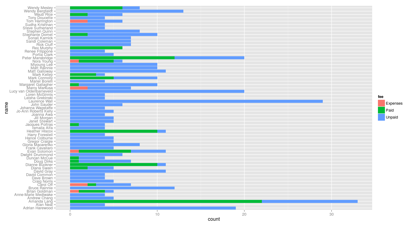
Lawrence Wall is doing a lot of unpaid appearances, and has never done any for pay. Good for him. Rex Murphy is the only busy person who only does paid appearances. Tells you something, that.
Let’s pick out just the paid appearances of the busy people. No need to colour anything this time.
> ggplot(busy %>% filter(fee == "Paid"), aes(name)) + geom_bar() + coord_flip()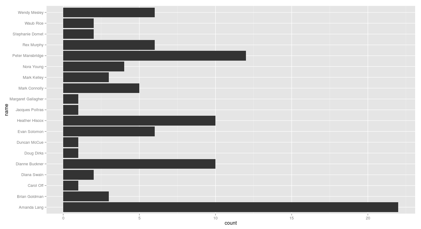
Amanda Lang is way out in the lead, with Peter Mansbridge second and Heather Hiscox and Dianne Buckner tied to show. In R, with dplyr, it’s easy to poke around in the data and see what’s going on, for example looking at the paid appearances of Amanda Lang and—as someone I’d expect/hope to be a lot different—Nora Young:
> busy %>% filter(name == "Amanda Lang", fee == "Paid") %>% select(date, event)
         date                                                                  event
1  2014-11-27                                            Productivity Alberta Summit
2  2014-11-26          Association of Manitoba Municipalities 16th Annual Convention
3  2014-11-24                               Portfolio Managers Association of Canada
4  2014-11-24                                           Sun Life Client Appreciation
5  2014-11-18                                            Vaughan Chamber of Commerce
6  2014-11-04                                       "PwC’s Western Canada Conference
7  2014-10-30 Chartered Institute of Management Accountants Conference on Innovation
8  2014-10-27                         2014 ASA - CICBV Business Valuation Conference
9  2014-10-22                                  Simon Fraser University Public Square
10 2014-10-07                        Colliers International Market Outlook Breakfast
11 2014-09-22                                          National Insurance Conference
12 2014-09-15                                                 RIMS Canada Conference
13 2014-08-19             Association of Municipalities of Ontario Annual Conference
14 2014-08-07                                      Manulife Asset Management Seminar
15 2014-07-10                                      Manulife Asset Management Seminar
16 2014-06-26                                      Manulife Asset Management Seminar
17 2014-05-29                                      Manulife Asset Management Seminar
18 2014-05-13                                             GeoConvention Show Calgary
19 2014-05-09                                    Alberta Urban Development Institute
20 2014-05-08                                          Young Presidents Organization
21 2014-05-07                                  Canadian Restaurant Investment Summit
22 2014-05-06                                   Canadian Hotel Investment Conference
> busy %>% filter(name == "Nora Young", fee == "Paid") %>% select(date, event)
        date                                                    event
1 2014-11-20          University of New Brunswick: Andrews initiative
2 2014-10-04 EdTech Team Ottawa: Bilingual Ottawa Summit feat. Google
3 2014-10-02               Humber College: President's Lecture Series
4 2014-10-01  Speech Ontario Professional Planners Institute: Healthy Communities and Planning in the Digital Age
Nora Young spoke about healthy communities and education to planners and colleges and universities … Amanda Lang spoke to developers and business groups and insurance companies. They are a lot different.
At this point, following up on any relation between Amanda Lang (or another host) and paid corporate gigs requires examination by hand. If the transcripts of The Exchange with Amanda Lang were available then it would be possible to write a script to look through them for mentions of these corporate hosts, which would provide clues for further examination. If the interviews were catalogued by a librarian with a controlled vocabulary then it would be even easier: you’d just do a query to find all occasions where (“Amanda Lang” wasPaidBy ?company) AND (“Amanda Lang” interviewed ?person) AND (?person isEmployeeOf ?company) and there you go, a list of interviews that require further investigation.
But it’s not all catalogued neatly, so journalists need to dig. This kind of initial data munging and visualization may, however, be helpful in pointing out who should be looked at first. Lang, Mansbridge and Murphy are the first three that Canadaland looked at, which does make me wonder what checking Hiscox and Buckner would show … are they different, and if so, how and why, and what does that say? I don’t know. This is as far as I’ll go with this cursory analysis.
In any case: hurrah to the CBC for making the data available, but boo for not making the raw data easy to use. Hurrah to Canadaland for investigating all this and forcing the issue.
Bakewell West Scales
Joan Bakewell interviews Prunella Scales and Timothy West is a fifteen-minute BBC radio interview, with journalist Joan Bakewell interviewing actors Prunella Scales and her husband Timothy West about Scales’s Alzheimer’s. You can hear it in evidence in what she says, but as sad as that is, the good humour of the two of them dealing with it—and all three of them dealing with old age—is remarkable. This is wonderful listening.
Bakewell: Do you remember Fawlty Towers?
Scales: Yes, what about—what do you mean, the lines?
Intersecting circles
A couple of months ago I was chatting about Venn diagrams with a nine-year-old (almost ten-year-old) friend named N. We learned something interesting about intersecting circles, and along the way I made some drawings and wrote a little code.
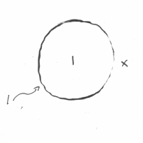
We started with two sets, but here let’s start with one. We’ll represent it as a circle on the plane. Call this circle c1.
Everything is either in the circle or outside it. It divides the plane into two regions. We’ll label the region inside the circle 1 and the region outside (the rest of the plane) x.
Now let’s look at two sets, which is probably the default Venn diagram everyone thinks of. Here we have two intersecting circles, c1 and c2.
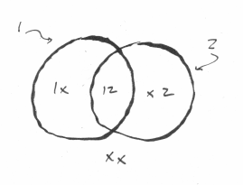
We need to consider both circles when labelling the regions now. For everything inside c1 but not inside c2, use 1x; for the intersection use 12; for what’s in c2 but not c1 use x2; and for what’s outside both circles use xx.
We can put this in a table:
| 1 | 2 |
|---|---|
| 1 | x |
| 1 | 2 |
| x | 2 |
| x | x |
This looks like part of a truth table, which of course is what it is. We can use true and false instead of the numbers:
| 1 | 2 |
|---|---|
| T | F |
| T | T |
| F | T |
| F | F |
It takes less space to just list it like this, though: 1x, 12, x2, xx.
It’s redundant to use the numbers, but it’s clearer, and in the elementary school math class they were using them, so I’ll keep with that.
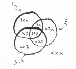
Three circles gives eight regions: 1xx, 12x, 1x3, 123, x2x, xx3, x23, xxx.
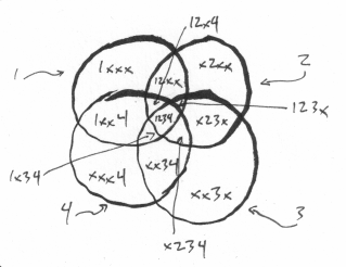
Four intersecting circles gets busier and gives 14 regions: 1xxx, 12xx, 123x, 12x4, 1234, 1xx4, 1x34, x2xx, x23x, x324, xx3x, xx34, xxx4, xxxx.
Here N and I stopped and made a list of circles and regions:
| Circles | Regions |
|---|---|
| 1 | 2 |
| 2 | 4 |
| 3 | 8 |
| 4 | 14 |
When N saw this he wondered how much it was growing by each time, because he wanted to know the pattern. He does a lot of that in school. We subtracted each row from the previous to find how much it grew:
| Circles | Regions | Difference |
|---|---|---|
| 1 | 2 | |
| 2 | 4 | 2 |
| 3 | 8 | 4 |
| 4 | 14 | 6 |
Aha, that’s looking interesting. What’s the difference of the differences?
| Circles | Regions | Difference | DiffDiff |
|---|---|---|---|
| 1 | 2 | ||
| 2 | 4 | 2 | |
| 3 | 8 | 4 | 2 |
| 4 | 14 | 6 | 2 |
Nine-year-old (almost ten-year-old) N saw this was important. I forget how he put it, but he knew that if the second-level difference is constant then that’s the key to the pattern.
I don’t know what triggered the memory, but I was pretty sure it had something to do with squares. There must be a proper way to deduce the formula from the numbers above, but all I could do was fool around a little bit. We’re adding a new 2 each time, so what if we take it away and see what that gives us? Let’s take the number of circles as n and the result as ?(n) for some unknown function ?.
| n | ?(n) |
|---|---|
| 1 | 0 |
| 2 | 2 |
| 3 | 3 |
| 4 | 12 |
I think I saw that 3 x 2 = 6 and 4 x 3 = 12, so n x (n-1) seems to be the pattern, and indeed 2 x 1 = 2 and 1 * 0 = 0, so there we have it.
Adding the 2 back we have:
Given n intersecting circles, the number of regions formed = n x (n - 1) + 2
Therefore we can predict that for 5 circles there will be 5 x 4 + 2 = 22 regions.
I think that here I drew five intersecting circles and counted up the regions and almost got 22, but there were some squidgy bits where the lines were too close together so we couldn’t quite see them all, but it seemed like we’d solved the problem for now. We were pretty chuffed.
When I got home I got to wondering about it more and wrote a bit of R.
I made three functions; the third uses the first two:
circle(x,y): draw a circle at (x,y), default radius 1.1roots(n): return the n nth roots of unity (when using complex numbers, x^n = 1 has n solutions)drawcircles(n): draw circles of radius 1.1 around each of those n roots
circle <- function(x, y, rad = 1.1, vertices = 500, ...) {
  rads <- seq(0, 2*pi, length.out = vertices)
  xcoords <- cos(rads) * rad + x
  ycoords <- sin(rads) * rad + y
  polygon(xcoords, ycoords, ...)
}

roots <- function(n) {
  lapply(
    seq(0, n - 1, 1),
    function(x)
      c(round(cos(2*x*pi/n), 4), round(sin(2*x*pi/n), 4))
  )
}

drawcircles <- function(n) {
  centres <- roots(n)
  plot(-2:2, type="n", xlim = c(-2,2), ylim = c(-2,2), asp = 1, xlab = "", ylab = "", axes = FALSE)
  lapply(centres, function (c) circle(c[[1]], c[[2]]))
}
drawcircles(2) does what I did by hand above (without the annotations):

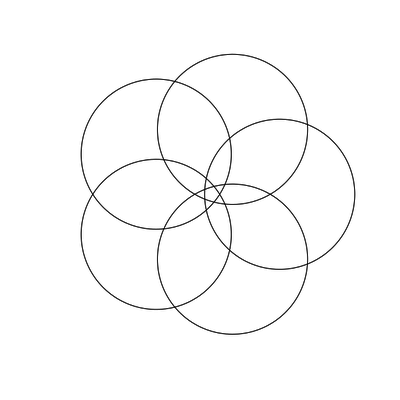
drawcircles(5) shows clearly what I drew badly by hand:
Pushing on, 12 intersecting circles:
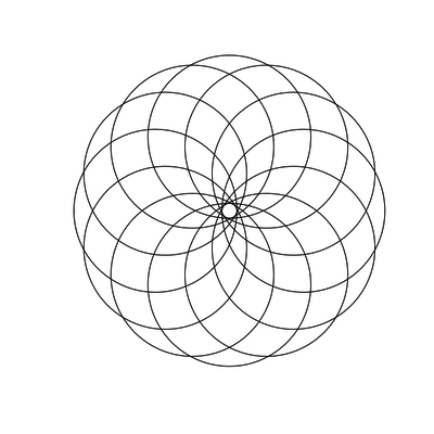
There are 12 x 11 + 2 = 123 regions there.
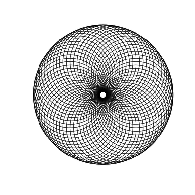
And 60! This has 60 x 59 + 2 = 3598 regions, though at this resolution most can’t be seen. Now we’re getting a bit op art.
This is covered in Wolfram MathWorld as Plane Division by Circles, and (2, 4, 8, 14, 24, …) is A014206 in the On-Line Encyclopedia of Integer Sequences: “Draw n+1 circles in the plane; sequence gives maximal number of regions into which the plane is divided.”
Somewhere along the way while looking into all this I realized I’d missed something right in front of my eyes: the intersecting circles stopped being Venn diagrams after 3!
A Venn diagram represents “all possible logical relations between a finite collection of different sets” (says Venn diagram on Wikipedia today). With n sets there are 2^n possible relations. Three intersecting circles divide the plane into 3 x (3 - 1) + 2 = 8 = 2^3 regions, but with four circles we have 14 regions, not 16! 1x3x and x2x4 are missing: there is nowhere where only c1 and c3 or c2 and c4 intersect without the other two. With five intersecting circles we have 22 regions, but logically there are 2^5 = 32 possible combinations. (What’s an easy way to calculate which are missing?)
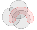
It turns out there are various ways to draw four- (or more) set Venn diagrams on Wikipedia, like this two-dimensional oddity (which I can’t imagine librarians ever using when teaching search strategies):
You never know where a bit of conversation about Venn diagrams is going to lead!
The sandbar
This metaphor for life and death from Pale Gray for Guilt (1968), one of John D. MacDonald’s Travis McGee novels, came to mind the other day. I looked it up, and here it is for easy reference.
Picture a very swift torrent, a river rushing down between rocky walls. There is a long, shallow bar of sand and gravel that runs right down the middle of the river. It is under water. You are born and you have to stand on that narrow, submerged bar, where everyone stands. The ones born before you, the ones older than you, are upriver from you. The younger ones stand braced on the bar downriver. And the whole long bar is slowly moving down that river of time, washing away at the upstream end and building up downstream.
Your time, the time of all your contemporaries, schoolmates, your loves and your adversaries, is that part of the shifting bar on which you stand. And it is crowded at first. You can see the way it thins out, upstream from you. The old ones are washed away and their bodies go swiftly by, like logs in the current. Downstream where the younger ones stand thick, you can see them flounder, lose footing, wash away. Always there is more room where you stand, but always the swift water grows deeper, and you feel the shift of the sand and the gravel under your feet as the river wears it away. Someone looking for a safer place can nudge you off balance, and you are gone. Someone who has stood beside you for a long time gives a forlorn cry and you reach to catch their hand, but the fingertips slide away and they are gone.
There are the sounds in the rocky gorge, the roar of the water, the shifting, gritty sound of sand and gravel underfoot, the forlorn cries of despair as the nearby ones, and the ones upstream, are taken by the current. Some old ones who stand on a good place, well braced, understanding currents and balance, last a long time. A Churchill, fat cigar atilt, sourly amused at his own endurance and, in the end, indifferent to rivers and the rage of waters. Far downstream from you are the thin, startled cries of the ones who never got planted, never got set, never quite understood the message of the torrent.