I happened to be looking at the xkcd About page and saw this, written by the comic’s creator Randall Munroe:
Is there an interface for automated systems to access comics and metadata?
Yes. You can get comics through the JSON interface, at URLs like https://xkcd.com/info.0.json (current comic) and https://xkcd.com/614/info.0.json (comic #614).
It also says:
xkcd.com updates without fail every Monday, Wednesday and Friday.
It’s always seemed so to me, but I felt like checking.
First, let’s get the data. Friday’s comic was number 2799, and we can fetch the JSON data for it with curl and format it with jq:
$ curl --silent https://xkcd.com/2799/info.0.json | jq
{
  "month": "7",
  "num": 2799,
  "link": "",
  "year": "2023",
  "news": "",
  "safe_title": "Frankenstein Claim Permutations",
  "transcript": "",
  "alt": "When I began trying to form a new claim by stitching together these parts in such an unnatural way, some called me mad.",
  "img": "https://imgs.xkcd.com/comics/frankenstein_claim_permutations.png",
  "title": "Frankenstein Claim Permutations",
  "day": "7"
}
jq is built for picking information out of JSON, like so:
$ curl --silent "https://xkcd.com/2799/info.0.json" | jq -r '[.year, .month, .day]'
[
  "2023",
  "7",
  "7"
]
Better yet, we can format it as CSV:
$ curl --silent "https://xkcd.com/2799/info.0.json" | jq -r '[.year, .month, .day]|@csv'
"2023","7","7"
The comics are numbered from 1–2799 without break, so we can fetch them with a looping shell script that gets each JSON file, picks out the data, and appends it to a file:
rm -f xkcd-dates.csv # Delete this file if it exists already
for i in $(seq 1 2799); do
	echo -n -e '\r' $i
	curl --silent "https://xkcd.com/${i}/info.0.json" | jq -r '[.year, .month, .day]|@csv' >> xkcd-dates.csv
	sleep 2
done
(The echo parameters show the number of the file being downloaded in a tidy way.)
When that’s done, we can fire up R. (Of course, we could have got the data in R, but a shell script is faster and easier for me.) Load in the tidyverse packages, then read the data and turn the raw date information stored into something more useful:
> library(tidyverse)
> xkcd <- read_csv("xkcd-dates.csv",
    col_names = c("year", "month", "day")) |>
    mutate(date = as.Date(paste0(year, "-", month, "-", day)),
    day_of_year = strftime(date, format = "%j"),
    week = strftime(date, format = "%V"),
    day_of_week = strftime(date, "%a"))
> xkcd
# A tibble: 2,798 × 7
    year month   day date       day_of_year week  day_of_week
   <dbl> <dbl> <dbl> <date>     <chr>       <chr> <chr>
 1  2006     1     1 2006-01-01 001         52    Sun
 2  2006     1     1 2006-01-01 001         52    Sun
 3  2006     1     1 2006-01-01 001         52    Sun
 4  2006     1     1 2006-01-01 001         52    Sun
 5  2006     1     1 2006-01-01 001         52    Sun
 6  2006     1     1 2006-01-01 001         52    Sun
 7  2006     1     1 2006-01-01 001         52    Sun
 8  2006     1     1 2006-01-01 001         52    Sun
 9  2006     1     1 2006-01-01 001         52    Sun
10  2006     1     1 2006-01-01 001         52    Sun
# ℹ 2,788 more rows
I don’t use day_of_year but I’ll leave it in there just in case.
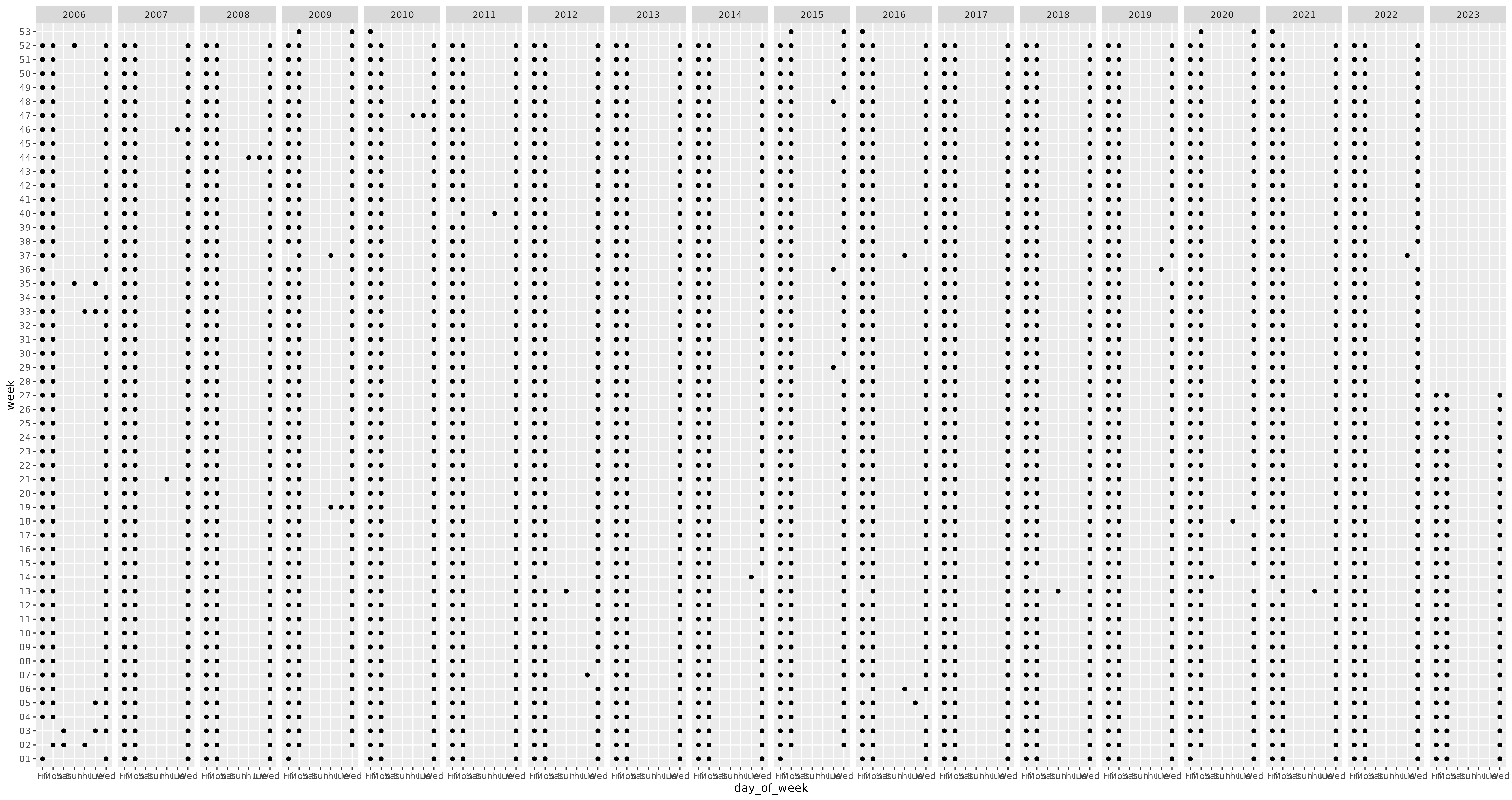
The first 44 comics are dated 2006-01-01, but we’ll ignore that. Try a quick chart (the image is a link that will show the image on its own, probably much larger):
> xkcd |> ggplot(aes(x = day_of_week, y = week)) + geom_point() + facet_grid(. ~ year)
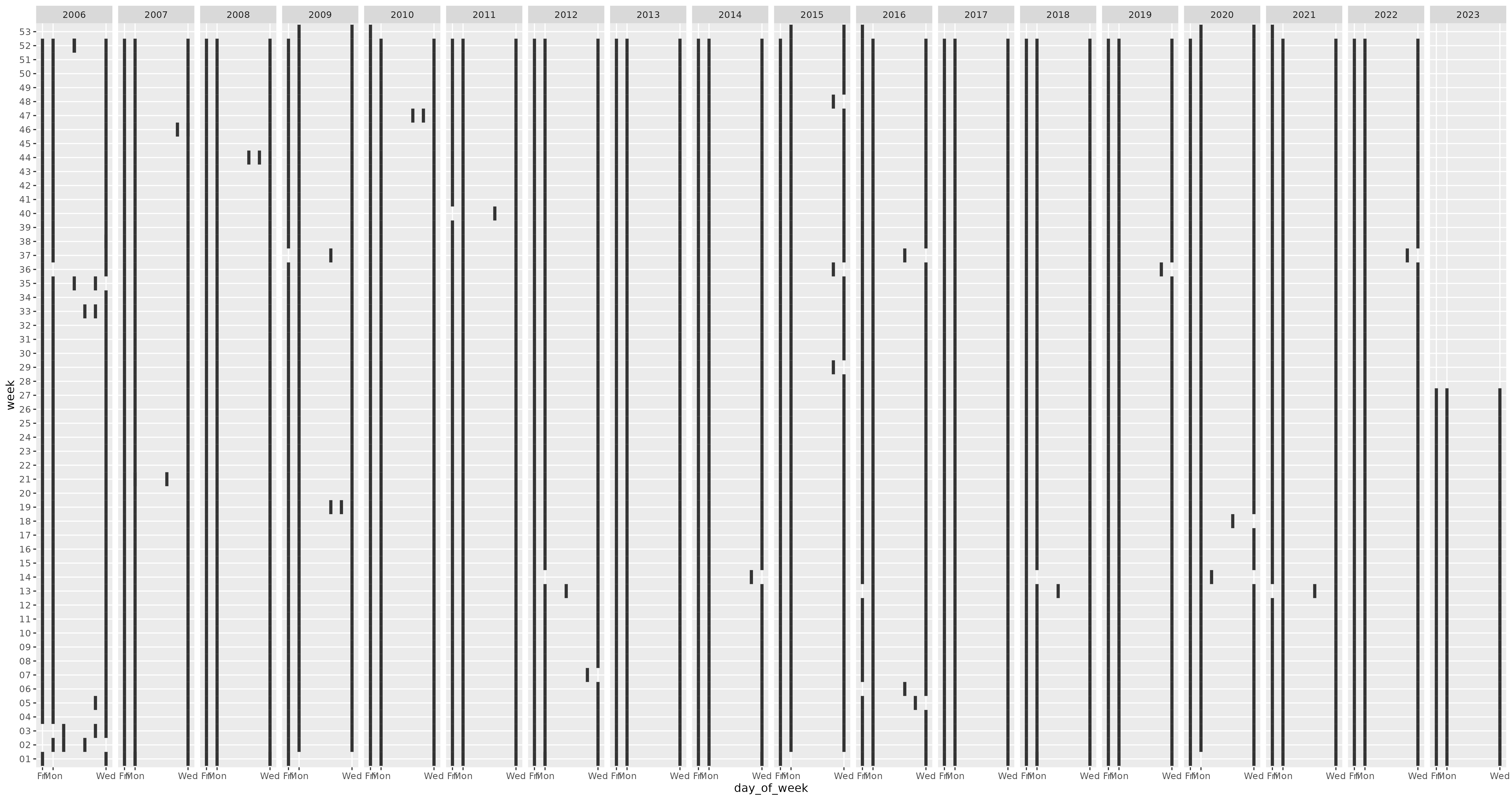
Looks very regular overall, with a few odd weeks here and there. Let’s tweak a few things:
> xkcd |> ggplot(aes(x = day_of_week, y = week)) +
    geom_tile(width = 0.3) +
    facet_grid(. ~ year) +
    scale_x_discrete(breaks = c("Mon", "Wed", "Fri"))
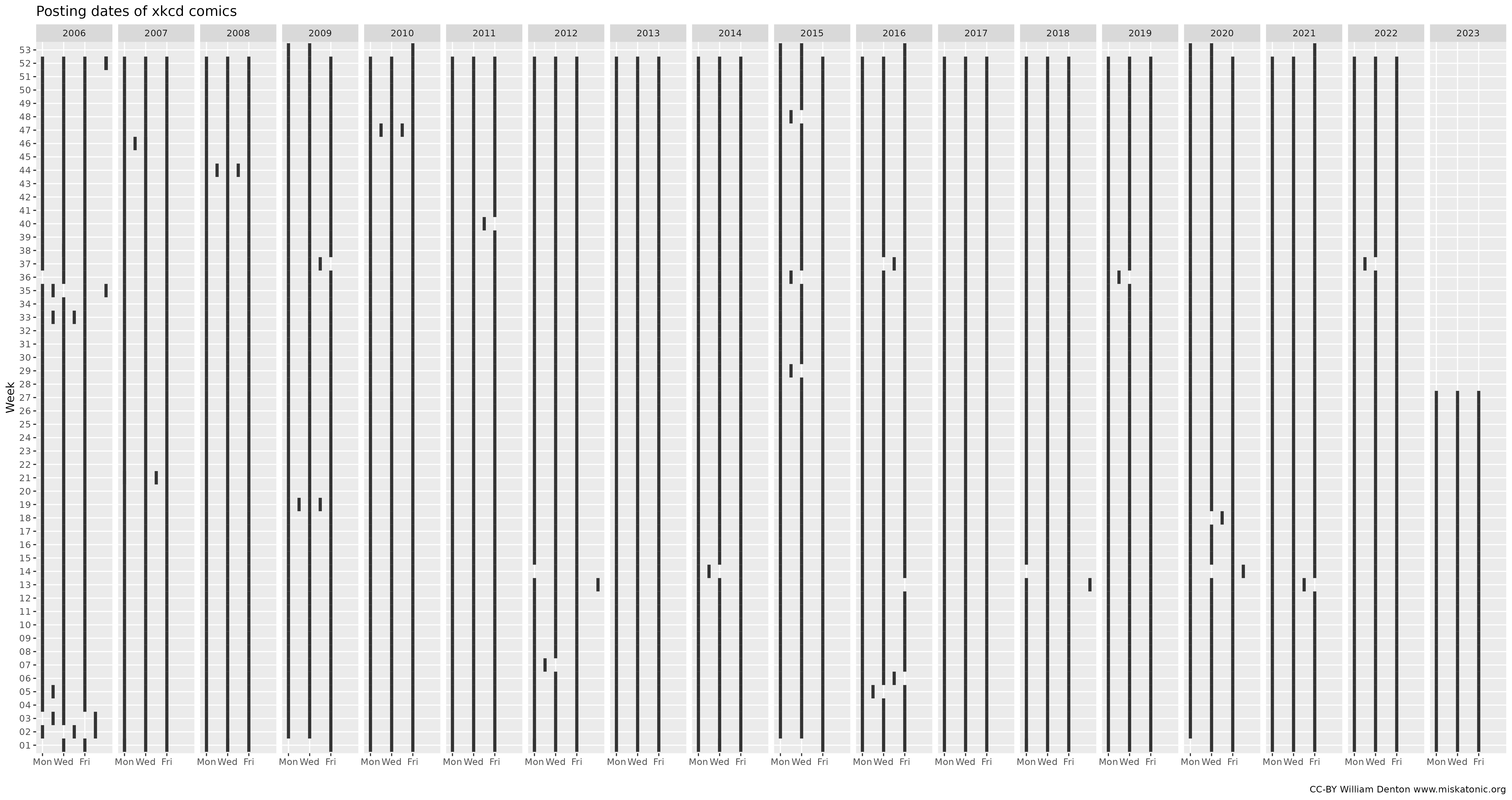
The days of the week aren’t plotting nicely, so we need to make the week start on Monday. Then fiddle a few more options to make a more finished chart.
> xkcd$day_of_week <- factor(xkcd$day_of_week, levels = c("Mon", "Tue", "Wed", "Thu", "Fri", "Sat", "Sun"))

> xkcd |> ggplot(aes(x = day_of_week, y = week)) + geom_tile(width = 0.3) + facet_grid(. ~ year) + scale_x_discrete(breaks = c("Mon", "Wed", "Fri")) + labs (x = "", y = "Week", title = "Posting dates of xkcd comics", caption = "CC-BY William Denton www.miskatonic.org")
At a glance it’s easy to see that (setting aside early 2006) Munroe overwhelmingly does post every Monday, Wednesday and Friday. There have been four weeks where he also posted on Tuesday and Thursday. It looks like there have been a number of weeks where he posted Wednesday’s comic on Tuesday. Maybe that’s a time zone thing. How many weeks have there been where he didn’t post three comics?
> xkcd |>
    count(year, week) |>
    filter(n < 3)
# #
# A tibble: 14 × 3
    year week      n
   <dbl> <chr> <int>
 1  2006 01        2
 2  2006 36        2
 3  2009 01        1
 4  2009 53        2
 5  2010 53        1
 6  2012 14        2
 7  2015 01        1
 8  2015 53        2
 9  2016 13        2
10  2016 53        1
11  2018 14        2
12  2020 01        2
13  2020 53        2
14  2021 53        1
Look at all those weeks numbered 01 or 53: those are partials at the beginning or end of a year. Ignore them. (To be sure about the counts, I should handle these weeks specially and sum across the entire week containing 01 January, but I can’t be bothered right now, so I’ll just ignore them. By eye it looks right.)
> xkcd |>
    count(year, week) |>
    filter(n < 3) |>
    filter(! week %in% c("01", "53"))
# # A tibble: 4 × 3
   year week      n
  <dbl> <chr> <int>
1  2006 36        2
2  2012 14        2
3  2016 13        2
4  2018 14        2
So it happened once each in 2006, 2012, 2016 and 2018. That’s dedication!
(I could have used the R package xkcd to make the charts look like an xkcd comic, but it requires installing a special font, and I couldn’t be bothered to do that either.)
Many thanks to Randall Munroe for providing the JSON files as well as his great comic.
 Miskatonic University Press