Sean Craig’s Amanda Lang took money from Manulife & Sun Life, gave them favourable CBC coverage piece on Canadaland got me looking at the cbcappearances script I wrote earlier this year.
It wasn’t getting any of the recent appearances—looks like the CBC changed how they are storing the data that is presented: instead of pulling it in on the fly from Google spreadsheets, it’s all the page in a hidden table (generated by their content management system, I guess) and shown as needed.
They should be making the data available in a reusable format, but they still aren’t. So we need to scrape it, but that’s easy, so I updated the script and regenerated appearances.csv, a nice reusable CSV file suitable for importing into your favourite data analysis tool. The last appearance listed was on 29 November 2014; I assume the December ones will show up soon in January.
The data shows 218 people have made 716 appearances since 24 April 2014. A quick histogram of appearances per person shows that most made only 1 or 2 appearances, and then it quickly tails off. Here how I did things in R:
> library(dplyr)
> library(ggplot2)
> cbc <- read.csv("appearances.csv", header = TRUE, stringsAsFactors = TRUE)
> cbc$date <- as.Date(cbc$date)
> totals <- cbc %>% group_by(name) %>% summarise(count = n()) %>% select(count)
> qplot(totals$count, binwidth = 1)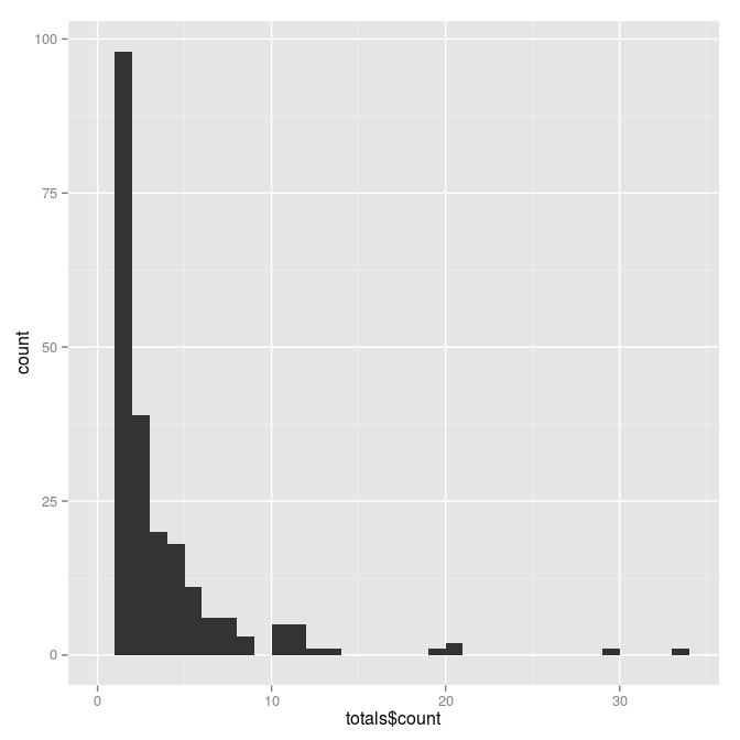
The median number of appearances is 2, the mean is about 3.3, and third quartile is 4 and above. Let’s label anyone in the third quartile as “busy,” and pick out everyone who is busy, then make a data frame of just the appearance information about busy people.
> summary(totals$count)
   Min. 1st Qu.  Median    Mean 3rd Qu.    Max.
  1.000   1.000   2.000   3.284   4.000  33.000
> quantile(totals$count)
  0%  25%  50%  75% 100%
  1    1    2    4   33
> busy.number <- quantile(totals$count)[[4]]
> busy.number
[1] 4
> busy_people <- cbc %>% group_by(name) %>% summarise(count = n()) %>% filter(count >= busy.number) %>% select(name)
> head(busy_people)
Source: local data frame [6 x 1]

                 name
1     Adrian Harewood
2           Alan Neal
3         Amanda Lang
4        Andrew Chang
5 Anne-Marie Mediwake
6       Brian Goldman
> busy <- a %>% filter(name %in% busy_people$name)
> head(busy)
   name             date                                           event       role      fee
1  Nora Young 2014-11-20 University of New Brunswick: Andrews initiative    Lecture     Paid
2  Carol Off  2014-11-14                                      War Museum  Interview Expenses
3  Rex Murphy 2014-11-13                              The Salvation Army     Speech     Paid
4  Carol Off  2014-11-03                                    Giller Prize  Interview     Paid
5  Carol Off  2014-11-01             International Federation of Authors  Interview   Unpaid
6  Carol Off  2014-10-27             International Federation of Authors  Interview   Unpaid
Now busy is a data frame of information about who did what where, but only for people with more than 4 appearances. It’s easy to do a stacked bar chart that shows how many of each type of fee (Paid, Unpaid, Expenses) each person received. There aren’t many situations where someone did a gig for expenses (red). Most are unpaid (blue) and some are paid (green).
> ggplot(busy, aes(name, fill = fee)) + geom_bar() + coord_flip()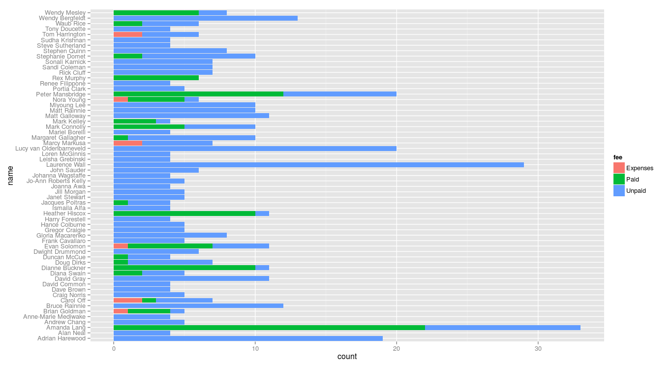
Lawrence Wall is doing a lot of unpaid appearances, and has never done any for pay. Good for him. Rex Murphy is the only busy person who only does paid appearances. Tells you something, that.
Let’s pick out just the paid appearances of the busy people. No need to colour anything this time.
> ggplot(busy %>% filter(fee == "Paid"), aes(name)) + geom_bar() + coord_flip()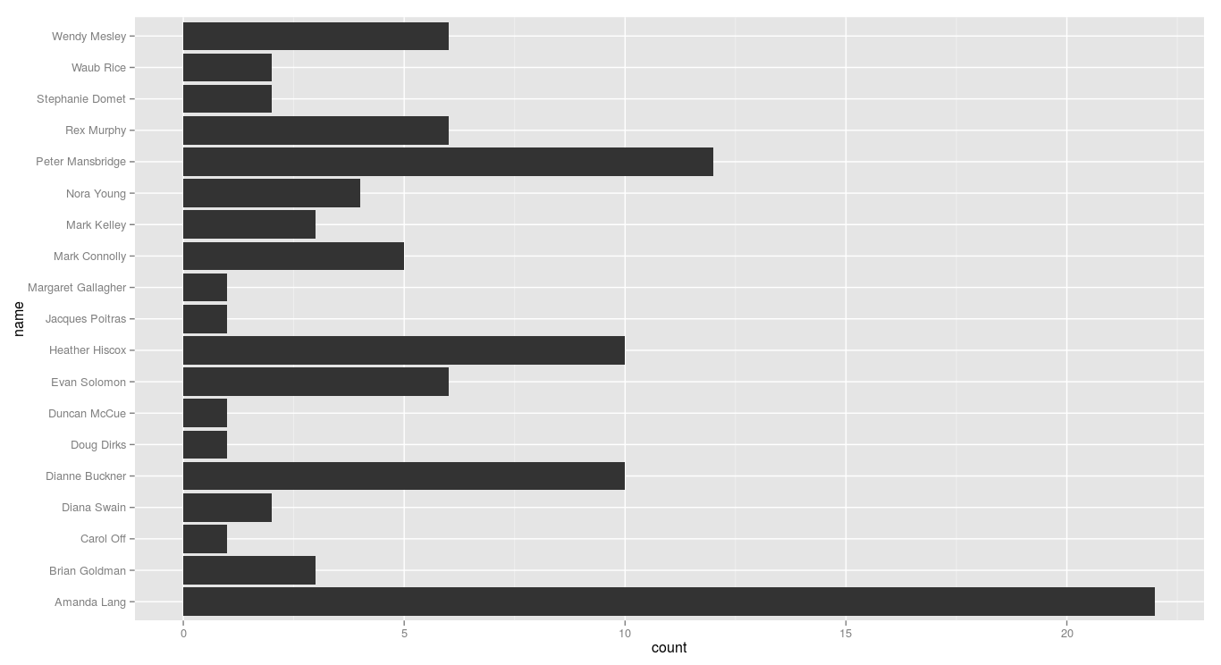
Amanda Lang is way out in the lead, with Peter Mansbridge second and Heather Hiscox and Dianne Buckner tied to show. In R, with dplyr, it’s easy to poke around in the data and see what’s going on, for example looking at the paid appearances of Amanda Lang and—as someone I’d expect/hope to be a lot different—Nora Young:
> busy %>% filter(name == "Amanda Lang", fee == "Paid") %>% select(date, event)
         date                                                                  event
1  2014-11-27                                            Productivity Alberta Summit
2  2014-11-26          Association of Manitoba Municipalities 16th Annual Convention
3  2014-11-24                               Portfolio Managers Association of Canada
4  2014-11-24                                           Sun Life Client Appreciation
5  2014-11-18                                            Vaughan Chamber of Commerce
6  2014-11-04                                       "PwC’s Western Canada Conference
7  2014-10-30 Chartered Institute of Management Accountants Conference on Innovation
8  2014-10-27                         2014 ASA - CICBV Business Valuation Conference
9  2014-10-22                                  Simon Fraser University Public Square
10 2014-10-07                        Colliers International Market Outlook Breakfast
11 2014-09-22                                          National Insurance Conference
12 2014-09-15                                                 RIMS Canada Conference
13 2014-08-19             Association of Municipalities of Ontario Annual Conference
14 2014-08-07                                      Manulife Asset Management Seminar
15 2014-07-10                                      Manulife Asset Management Seminar
16 2014-06-26                                      Manulife Asset Management Seminar
17 2014-05-29                                      Manulife Asset Management Seminar
18 2014-05-13                                             GeoConvention Show Calgary
19 2014-05-09                                    Alberta Urban Development Institute
20 2014-05-08                                          Young Presidents Organization
21 2014-05-07                                  Canadian Restaurant Investment Summit
22 2014-05-06                                   Canadian Hotel Investment Conference
> busy %>% filter(name == "Nora Young", fee == "Paid") %>% select(date, event)
        date                                                    event
1 2014-11-20          University of New Brunswick: Andrews initiative
2 2014-10-04 EdTech Team Ottawa: Bilingual Ottawa Summit feat. Google
3 2014-10-02               Humber College: President's Lecture Series
4 2014-10-01  Speech Ontario Professional Planners Institute: Healthy Communities and Planning in the Digital Age
Nora Young spoke about healthy communities and education to planners and colleges and universities … Amanda Lang spoke to developers and business groups and insurance companies. They are a lot different.
At this point, following up on any relation between Amanda Lang (or another host) and paid corporate gigs requires examination by hand. If the transcripts of The Exchange with Amanda Lang were available then it would be possible to write a script to look through them for mentions of these corporate hosts, which would provide clues for further examination. If the interviews were catalogued by a librarian with a controlled vocabulary then it would be even easier: you’d just do a query to find all occasions where (“Amanda Lang” wasPaidBy ?company) AND (“Amanda Lang” interviewed ?person) AND (?person isEmployeeOf ?company) and there you go, a list of interviews that require further investigation.
But it’s not all catalogued neatly, so journalists need to dig. This kind of initial data munging and visualization may, however, be helpful in pointing out who should be looked at first. Lang, Mansbridge and Murphy are the first three that Canadaland looked at, which does make me wonder what checking Hiscox and Buckner would show … are they different, and if so, how and why, and what does that say? I don’t know. This is as far as I’ll go with this cursory analysis.
In any case: hurrah to the CBC for making the data available, but boo for not making the raw data easy to use. Hurrah to Canadaland for investigating all this and forcing the issue.