This is the fifth and last in a series about using R to look at reference desk statistics recorded in LibStats. Previously:
- Ref desk 1: LibStats
- Ref desk 2: Questions asked per week at a branch
- Ref desk 3: Comparing question.type across branches
- Ref desk 4: Calculating hours of interactions
I've been making some other charts showing other kinds of ratios and calculations but I'm going to skip to one last pair of charts where I bring in the number of our students to figure out how many students we help with research help each week and for how long.
First, a brief review of the four branches of the York University Libraries system we're looking at:
- Scott is arts, humanities and social sciences, and the building includes the map library, the archives, and music/film library
- Bronfman is business
- Frost is on the Glendon campus in another part of the city and handles all of the students there
- Steacie is science, engineering and health
(Osgoode is law but they don't use LibStats so we'll forget about them for now.)
I calculated how many "home students" each library has. Bronfman handles everyone in the business school and in the administrative studies program in another faculty. Steacie handles everyone in the science and health faculties (except psychology, which is handled at Scott). Frost handles everyone at Glendon. Scott handles everyone else. The York University Factbook let me look up how many students were in each faculty, and I did a bit of adding and subtracting and figured out:
- Scott has 34,388 "home students"
- Bronfman has 6,050
- Frost has 2,677
- Steacie has 10,018
That's 53,133 students total, as of last fall. (We have about 43 librarians and archivists, for a ratio of 1235 students to each librarian, which is one of the worst in Canada.)
You can figure out something very similar for your library, probably.
With those numbers, we're all set for some more work in R.
First, I make a libstats.bigscott data frame, which gloms together all of the reference desk activities that happen in the Scott Library building (which as I said contains three smaller libraries) into one. This is necessary to group together all possible arts/humanities/social sciences questions. These lines below rename certain library.name fields by saying, for example for SMIL, for every entry in this data frame where library.name equals "SMIL", make library.name equal "Scott." Nice example of vector thinking in R.
> libstats.bigscott <- libstats
> libstats.bigscott$library.name[libstats.bigscott$library.name == "SMIL"] <- "Scott"
> libstats.bigscott$library.name[libstats.bigscott$library.name == "ASC"] <- "Scott"
> libstats.bigscott$library.name[libstats.bigscott$library.name == "Maps"] <- "Scott"
> libstats.bigscott$week <- as.Date(cut(as.Date(libstats.bigscott$timestamp, format="%m/%d/%Y %r"), "week", start.on.monday=TRUE))
Next, use our old friend ddply to count how many research questions are asked each week.
> research.users <- ddply(subset(libstats.bigscott,
                                 question.type %in% c("4. Strategy-Based", "5. Specialized")),
                          .(library.name, week), nrow)
> names(research.users)[3] <- "users"
> research.users$user.ratio <- NA
> head(research.users)
> library.name       week users user.ratio
1     Bronfman 2011-01-31    48         NA
2     Bronfman 2011-02-07    80         NA
3     Bronfman 2011-02-14    42         NA
4     Bronfman 2011-02-21    61         NA
5     Bronfman 2011-02-28    53         NA
6     Bronfman 2011-03-07    59         NA
Now, another probably heinous non-R way of dividing the number of users (or, actually, questions) each week by the number of "home students":
> for (i in 1:nrow(research.users)) {
    if (research.users[i,1] == "Bronfman"          ) { research.users[i,4] = research.users[i,3] / 6050  }
    if (research.users[i,1] == "Frost"             ) { research.users[i,4] = research.users[i,3] / 2677  }
    if (research.users[i,1] == "Scott"             ) { research.users[i,4] = research.users[i,3] / 34388 }
    if (research.users[i,1] == "Steacie"           ) { research.users[i,4] = research.users[i,3] / 10018 }
  }
> library.name       week users  user.ratio
1     Bronfman 2011-01-31    48 0.007933884
2     Bronfman 2011-02-07    80 0.013223140
3     Bronfman 2011-02-14    42 0.006942149
4     Bronfman 2011-02-21    61 0.010082645
5     Bronfman 2011-02-28    53 0.008760331
6     Bronfman 2011-03-07    59 0.009752066
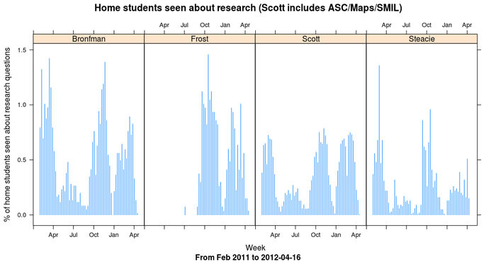
user.ratio there is what we're after. It looks low, doesn't it? Multiply it by 100 to get a percentage. It's still low.

The y-axis is per cent, so this shows that usually through term time we see give research help to under 1% of our students. There are a few weeks in some branches where it gets above that, but it's never above 1.5%.
That really surprised me. I have no idea what the numbers are like at other universities. If you figure it out for where you work, let me know. Perhaps one per cent is a common figure? Could it be five per cent at some universities? It would have to be a small university, I think, or have a lot of librarians.
Know that we know how many students we help with research, I wondered how long we spend helping them. More calculations in R, using ref.desk.spent, the function I defined in the last post to add up an estimate of how much time is spent at the desk. Here we break it down by branch by week, create a research.time.bigscott data frame, which I then merge with research.users so I can divide to create the research.mins.ratio which is what I'm after:
> research.time.bigscott <- data.frame(library.name = factor(), week = factor(), research.mins = numeric())
> branches <- c("Scott", "Frost", "Bronfman", "Steacie")
> for (i in 1:length(branches)) {
    branchname <- branches[i]
    for (j in 1:length(weeks)) {
      spent <- desk.time.spent(ddply(subset(libstats.bigscott,
                                            library.name == branchname & week==weeks[j] &
                                            question.type %in% c("4. Strategy-Based", "5. Specialized")),
                                     .(time.spent), nrow))
      rbind(research.time.bigscott,
            data.frame(library.name = branchname, week = weeks[j], research.mins = spent)) -> research.time.bigscott
    }
  }
> research.users$week <- as.factor(research.users$week) # Necessary for merge to work cleanly
> research.time.bigscott <- merge(research.time.bigscott, research.users, by=c("library.name", "week"))
> research.time.bigscott$research.mins.ratio <- research.time.bigscott$research.mins / research.time.bigscott$users
> head(research.time.bigscott)
  library.name       week research.mins users  user.ratio research.mins.ratio
1     Bronfman 2011-01-31           758    48 0.007933884            15.79167
2     Bronfman 2011-02-07          1340    80 0.013223140            16.75000
3     Bronfman 2011-02-14           595    42 0.006942149            14.16667
4     Bronfman 2011-02-21           997    61 0.010082645            16.34426
5     Bronfman 2011-02-28           775    53 0.008760331            14.62264
6     Bronfman 2011-03-07           901    59 0.009752066            15.27119
> xyplot(research.mins.ratio ~ as.Date(week) | library.name, data = research.time.bigscott,
         type = "h",
         ylab = "Length of average research interaction (minutes)",
         xlab = "Week",
         main = "Average length of research interactions (Scott includes ASC/Maps/SMIL)",
         sub = paste("From Feb 2011 to", up.to.week),
         abline=list(h=15, lty=3, col="lightgrey"),
        )
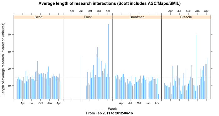
In this xyplot command I throw in an extra abline to draw a dashed light grey line along y=15 to help point out that generally we spend about fifteen minutes on each research interaction.

The Steacie library stands out from the others, and there are some peaks here and there, but overall we spend on average about fifteen minutes on each research interaction with students.
Put those two charts together and it shows that during term time we spend on average about fifteen minutes a week giving research help to each of under one per cent of our students.
 Miskatonic University Press