(Fourth in a series about using R to look at reference desk statistics recorded in LibStats. Third was Ref desk 3: Comparing question.type across branches.)
The last two posts looked at two straightforward breakdowns of reference desk activity at a library with several branches: questions by branch (to look at all activity at a single branch) and branches by question (to compare how many questions of the same type are asked at all branches). Both are very useful and lead to interesting questions and discussions. I'm sticking to numbers and charts here, but they are just the beginning of a larger discussion about the purpose of the reference desk is and how it works at a library---and how reference desk statistics are recorded, and what the act of recording means.
It's important to talk about all of that, and I do enjoy those discussions. But right now I'm going to make another chart.
Another fact we record about each reference desk interaction is its duration, which in our libstats data frame is in the time.spent column. As I explained in Ref Desk 1: LibStats, these are the options:
- NA ("not applicable," which I've used, though I can't remember why)
- 0-1 minute
- 1-5 minutes
- 5-10 minutes
- 10-20 minutes
- 20-30 minutes
- 30-60 minutes
- 60+ minutes
We can use this information to estimate the total amount of time we spend working with people at the desk: it's just a matter of multiplying the number of interactions by their duration.
Except we don't know the exact length of each duration, we only know it with some error bars: if we say an interaction took 5-10 minutes then it could have taken 5, 6, 7, 8, 9, or 10 minutes. 10 is 100% more than 5: relatively that's a pretty big range. (Of course, mathematically it makes no sense to have a 5-10 minute range and a 10-20 minute range, because if something took exactly 10 minutes it could go in either category.)
Let's make some generous estimates about a single number we can assign to the duration of reference desk interactions.
| Duration | Estimate |
|---|---|
| NA | 0 minutes |
| 0-1 minute | 1 minute |
| 1-5 minutes | 5 minutes |
| 5-10 minutes | 10 minutes |
| 10-20 minutes | 15 minutes |
| 20-30 minutes | 25 minutes |
| 30-60 minutes | 40 minutes |
| 60+ minutes | 65 minutes |
This means that if we have 10 transactions of duration 1-5 minutes we'll call it 10 * 5 = 50 minutes total. If we have 10 transactions of duration 20-30 minutes we'll call it a 10 * 25 = 250 minutes total. These estimates are arguable but I think they're good enough. They're on the generous side for the shorter durations, which make up most of the interactions.
Next, we need to figure out how many interactions happened of each possible duration. This is easily done using ddply as we did before, but this time to count by time.spent:
> tmp <- ddply(libstats, .(time.spent, week), nrow)
> head(tmp)
  time.spent       week   V1
1 0-1 minute 2011-01-31  811
2 0-1 minute 2011-02-07 1220
3 0-1 minute 2011-02-14 1177
4 0-1 minute 2011-02-21  592
5 0-1 minute 2011-02-28  949
6 0-1 minute 2011-03-07 1037
This tells us that across our library system in the week starting 2011-01-31 there were 811 interactions that took 0-1 minutes. What else happened that week? How many interactions were there of all other durations?
> subset(tmp, week == " 2011-01-31")
       time.spent       week  V1
1      0-1 minute 2011-01-31 811
65    1-5 minutes 2011-01-31 299
129 10-20 minutes 2011-01-31  72
212 20-30 minutes 2011-01-31  28
274 30-60 minutes 2011-01-31   6
332  5-10 minutes 2011-01-31 153
447          <NA> 2011-01-31  11
What's the total amount of time spent dealing with people at the desk? We'll use our rule defined above, and just ignore the NAs:
> 811*1 + 299*5 + 72*15 + 28*25 + 6*40 + 153*10
[1] 5856
> round(5856/60)
[1] 98
Answer: about 98 hours.
That's just one week, though. How can we figure it out for each week, and then chart that? I'd hoped to be able to do it in a nice R way with one of the apply functions, because I was in exactly the situation that Neil Saunders describes in A brief introduction to "apply" in R:
At any R Q&A site, you'll frequently see an exchange like this one:
Q: How can I use a loop to [...insert task here...] ?
A: Don't. Use one of the apply functions.
I'd hoped to go at it with some kind of arrangement with a data frame of duration factors and estimated times:
     duration       estimate
   0-1 minute              1
  1-5 minutes              5
 5-10 minutes             10
10-20 minutes             15
20-30 minutes             25
30-60 minutes             40
  60+ minutes             60
Then I'd apply a function to each row of tmp that would check the value of time.spent, look up the equivalent duration in this data frame to find the estimate that goes with it, multiply V1 * estimate and then put the result in an interaction.time column. I took a stab at but couldn't get it working, so I did it with a loop. It's not the R way, but it worked, and I'll take another crack at it another day.
So to do it the ugly way, first I define a function:
> desk.time.spent <- function(x) {
    if (nrow(x) == 0) { return(0) }
    sum = 0
    for (i in 1:nrow(na.omit(x))) {
      if      (x[i,1] == "0-1 minute"   ) { sum = sum + 1 * x[i,2]  }
      else if (x[i,1] == "1-5 minutes"  ) { sum = sum + 5 * x[i,2]  }
      else if (x[i,1] == "5-10 minutes" ) { sum = sum + 10 * x[i,2]  }
      else if (x[i,1] == "10-20 minutes") { sum = sum + 15 * x[i,2] }
      else if (x[i,1] == "20-30 minutes") { sum = sum + 25 * x[i,2] }
      else if (x[i,1] == "30-60 minutes") { sum = sum + 40 * x[i,2] }
      else if (x[i,1] == "60+ minutes"  ) { sum = sum + 65 * x[i,2] }
    }
    return(sum)
  }
Then I create an empty data frame and reset which branches to look at, just in case I fiddled that somewhere before:
> interaction.time <- data.frame(library.name = factor(), week = factor(), desk.mins = numeric())
> interaction.time$week = as.Date(interaction.time$week) # Can't set this in the line above
> branches <- levels(libstats$library.name)
Then I loop through the branches, using ddply to calculate how many of each question was asked each week, and passing that data frame to the desk.time.spent() function for multiplication. It returns the number of minutes spent that week helping people, and then rbind matches things up to add a new row to the interaction.time data frame.
> for (i in 1:length(branches)) {
    branchname <- branches[i]
    write (branchname, stderr())
    for (j in 1:length(weeks)) {
      spent <- desk.time.spent(ddply(subset(libstats,
    library.name == branchname & week==weeks[j]), .(time.spent), nrow))
      rbind(interaction.time,
        data.frame(library.name = branchname, week = weeks[j], desk.mins = spent)) -> interaction.time
    }
  }
> tail(interaction.time)
    library.name       week desk.mins
429      Steacie 2012-02-27      1460
430      Steacie 2012-03-05      1180
431      Steacie 2012-03-12      1110
432      Steacie 2012-03-19      1286
433      Steacie 2012-03-26      1042
434      Steacie 2012-04-02      1523
(desk.mins is actually time spent not only at the desk but in offices and anywhere else. Just ignore the name, or change it---I'm copying this from a script that does something slightly different.)
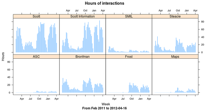
> xyplot(desk.mins/60 ~ as.Date(week)|library.name, data = interaction.time,
         type = "h",
         ylab = "Hours",
         xlab = "Week",
         main = "Hours of interactions",
         sub = paste("From Feb 2011 to", up.to.week),
        )

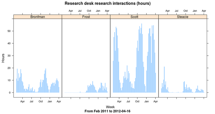
Let's narrow things down and look at only research questions (4s and 5s) at the reference desk. Librarians and archivists often help people with research questions in an office, not at the desk---such practices vary from library to library and discipline to discipline, and of course not all branches have reference/research desks---and those aren't counted here. Nevertheless, it's an interesting view on what happens at the desk, and it's an instructive example about how to slice the data more finely, but as always we have to remember what data is being shown.
> branches <- c("Bronfman", "Frost", "Scott", "Steacie")
> research.interaction.time <- data.frame(library.name = factor(), week = factor(), research.mins = numeric())
> for (i in 1:length(branches)) {
    branchname <- branches[i]
    write (branchname, stderr())
    for (j in 1:length(weeks)) {
      spent <- desk.time.spent(ddply(subset(libstats,
                                          library.name == branchname & week==weeks[j] &
                                          location.name %in% c("Consultation Desk", "Drop-in Desk", "Reference Desk") &
                                          question.type %in% c("4. Strategy-Based", "5. Specialized")
                                          ),
                                   .(time.spent), nrow))
      rbind(research.interaction.time, data.frame(library.name = branchname, week = weeks[j],
      research.mins = spent)) -> research.interaction.time
    }
  }
> interaction.time <- merge(interaction.time, research.interaction.time, by=c("week", "library.name"))
> tail(interaction.time)
          week library.name desk.mins research.mins
243 2012-03-26        Scott      2856          1946
244 2012-03-26      Steacie      1042           110
245 2012-04-02     Bronfman       781           270
246 2012-04-02        Frost       351            55
247 2012-04-02        Scott      1467           960
248 2012-04-02      Steacie      1523            20
> xyplot(research.mins/60 ~ as.Date(week) | library.name, data = interaction.time,
         type = "h",
         ylab = "Hours",
         xlab = "Week",
         main = "Research desk research interactions (hours)",
         sub = paste("From Feb 2011 to", up.to.week),
        )

In the next post, the last of this short series, I'll bring in the number of students and do a couple of calculations based on that.
 Miskatonic University Press